Topics (384k) Articles (398k) Users (410) Discussions (242) Comments (383) Files (13k) New article

A normal Q-Q plot compares order statistics with standard normal quantiles . For a normal distribution with , the population quantile function is , so the diagnostic sample relation isThe appropriate reference is a line with an intercept and positive slope, not necessarily the identity line. A line can be fitted through two central sample quantiles; R's
qqline uses the quantile levels and by default. Neither that line nor its fitting rule is part of the definition of a normal Q-Q plot. [ref]https://stat.ethz.ch/R-manual/R-devel/library/stats/html/qqnorm.html. R stats documentation, qqnorm and qqline
To isolate curvature, retain the same 19 plotting positions and construct two more ordered sequences:The are continuous uniform distribution quantiles on , while the apply the hyperbolic sine to the reference quantiles. Both examples are symmetric about zero. At ranks , is approximately and is approximately . Again, these are constructed values rather than random draws or real data.
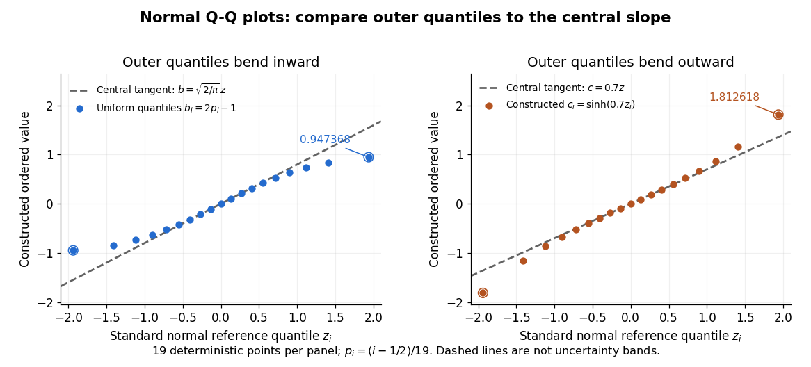
Read these shapes relative to their central slope. The uniform distribution example has , with derivative ; at the upper endpoint the tangent predicts , while . Its lower end lies above the tangent and its upper end below it: the outer quantiles are compressed. The hyperbolic sine example has ; its tangent predicts at the upper endpoint, while . Its lower end lies below the tangent and its upper end above it: the outer quantiles are stretched. Unequal departures at the two ends can suggest skewness. The direction of these descriptions assumes that reference quantiles are horizontal and observed values vertical. The graphs illustrate finite-range shape differences; a sample pattern cannot establish an asymptotic tail probability law or membership in a heavy-tailed distribution class.
A nearly straight normal Q-Q plot is a diagnostic, not a proof of a normal distribution or a formal hypothesis test. Random statistical samples fluctuate, particularly at extreme order statistics, and apparent curvature depends on sample size, plotting positions and the reference line. A calibrated hypothesis test or uncertainty band requires its own assumptions and must account for parameters estimated from the same observations. Sorting also discards the original observation order: rearranging a time series leaves its Q-Q plot unchanged, so the plot cannot establish independence.
For a normal linear model, R's diagnostic normal Q-Q plot uses standardized regression residuals, also called internally studentized residuals. [ref]
https://stat.ethz.ch/R-manual/R-devel/library/stats/html/plot.lm.html. Maindonald and Maechler, R plot.lm documentation, Details
Even with independent errors, the regression residuals have covariance matrix , where is the hat matrix; fitting parameters generally creates dependencies. Dividing by a shared estimated standard deviation creates further dependence, and the distribution of an internally studentized Gaussian residual is not exactly the standard normal distribution. The normal Q-Q plot therefore helps assess error shape alongside other diagnostics rather than certifying independent normal random variables.For a bipartite vector and a chosen orthonormal basis of , the generally unnormalized relative state on is obtained by the partial inner product with one basis vector. It gives the expansion . The squared norm of a relative state is the probability of its corresponding basis outcome when is normalized. Relative states of eigenvectors of a Choi matrix construct the columns of its Kraus operators.
The 1953 paper The isolation of protoplasts from Bacillus megaterium by controlled treatment with lysozyme by Claes Weibull (pp. 688–690, Figures 2–3) tested Bacillus megaterium strain KM. Apparatus included a Klett-Summerson colorimeter with a red filter and a Spencer no. 8 phase-contrast microscope. Lysozyme in phosphate buffer produced empty residual bodies; adding sucrose preserved granular spheres. Diluting their surroundings caused rapid osmotic lysis.
The same study compared untreated, boiled, lysozyme-exposed and sucrose-protected samples. Filled, stoppered tubes reduced damage from air exposure. After centrifugation, a Beckman DU spectrophotometer measured ultraviolet wave absorption of the separated liquid. Protected samples resembled untreated controls in releasing little ultraviolet-absorbing material; boiled and unprotected samples released much more. Later-growth cultures reduced spontaneous breakdown as a confounder.[ref]
The isolation of protoplasts from Bacillus megaterium by controlled treatment with lysozyme by Claes Weibull. pp. 688–689, Materials and Methods; pp. 692–694, release comparison and Figure 6
Together, the shape and release readouts support removal of mechanical protection while a permeability barrier persists. They do not establish unchanged selective permeability to every solute, long-term viability, or universal susceptibility.
An instructive extension of this experimental logic is a matched comparison: lysozyme present or absent, crossed with osmotic support present or absent. Keep starting material, buffer, observation interval and handling comparable; include a blank to distinguish optical effects of reagents from changes in the biological cells. Then dilute already formed protoplasts as a separate intervention. This separates access and wall removal from failure after removal. These are proposed controls for interpreting the mechanism, not additional reported results from the historical paper. A fall in optical signal alone cannot establish rupture: shape changes also alter scattering of light.
A protein disulfide bond is a disulfide bond linking two sulfur chemical atoms carried by suitable amino acid residues. It can connect distant portions of a polypeptide chain or different chains. See Cooper: sulfur-containing residues and disulfide crosslinks. The four internal protein disulfide bonds of ribonuclease A are central to the ribonuclease A refolding experiment; breaking these crosslinks need not break the peptide bonds along its protein backbone.
A protein binding site is a region of a protein structure that interacts with a ligand. Its arrangement of amino acid residues helps determine recognition; connecting loops supported by a beta sheet can contribute to it. An enzyme's active site binds a substrate and accelerates a chemical reaction. See Alberts et al.: protein binding sites and active sites.
A backbone hydrogen bond is a hydrogen bond involving groups of the protein backbone, typically a backbone oxygen chemical atom and a hydrogen chemical atom already joined by a covalent bond to backbone nitrogen. It can connect positions that are not adjacent along the polypeptide chain. The peptide bonds still determine which amino acid residues are consecutive. See the original structural argument cited under alpha helix.
A beta sheet consists of extended stretches of protein backbone lying alongside one another, joined by backbone hydrogen bonds. The stretches can belong to different portions of the same polypeptide chain or to different chains.
Each extended stretch is a beta strand. Neighboring beta strands pack side by side, with repeated backbone hydrogen bonds between their backbone and groups: the oxygen is a hydrogen bond acceptor, and the backbone nitrogen with its attached hydrogen provides a hydrogen bond donor. These are interactions of the shared protein backbone, not merely contacts between amino acid side chains. Unlike an alpha helix, a beta sheet joins adjacent extended stretches rather than coiling one stretch around an axis. See Clark, Douglas and Choi, Biology 2e, 3.4: backbone groups in secondary structure.
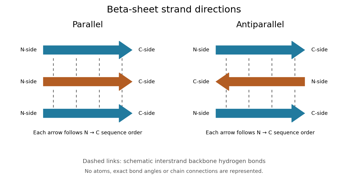
Read each beta strand in the sequence direction from the N-terminus toward the C-terminus, even when it is an internal part of a longer polypeptide chain. In a parallel beta sheet, neighboring beta strands run in the same N→C direction; in an antiparallel beta sheet, they run in opposite N→C directions. A three-strand example can therefore have arrows right–right–right or right–left–right. A beta sheet can also mix the two arrangements. Direction does not identify chain membership: a single polypeptide chain can fold back to supply several beta strands, and different polypeptide chains can contribute to one beta sheet. See Alberts et al., Molecular Biology of the Cell: beta-sheet strand arrangements.
The pleated appearance comes from the geometry of the protein backbone. Successive amino acid residues carry amino acid side chains on alternating faces of an ideal beta strand, conventionally drawn above and below the sheet. The attachment positions are the amino acid alpha carbons. Thus a six-position cartoon has groups 1, 3 and 5 on one face and 2, 4 and 6 on the other. This alternation is a spatial pattern, not a rule that alternating positions must contain identical amino acids. See Clark, Douglas and Choi: side chains above and below the pleats.
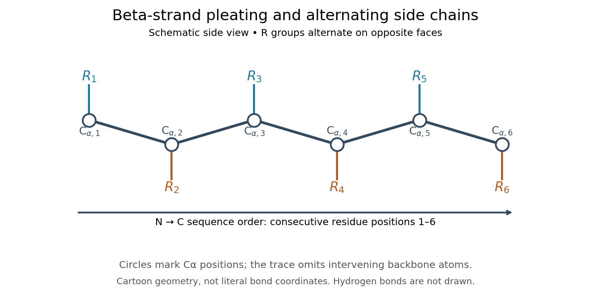
Real beta sheets commonly twist and curve; pleating does not make them perfectly flat plates. Which beta strands are neighbors, how connecting regions join them, and how their faces pack are features of the three-dimensional protein structure. An alternating pattern in the protein primary structure alone neither establishes a beta sheet nor specifies a unique fold independently of surroundings and interacting molecules. See Breda et al., Protein Structure, Modelling and Applications: extended strands, sheet twist and three-dimensional organization and protein folding.
Why this arrangement is useful: repeated backbone hydrogen bonds organize extended chain regions into a framework that can contribute to the interior of a folded protein. Amino acid side chains and connecting loops give that framework chemical variety and can shape a protein binding site for a ligand. Its attractive feature is the combination of a reusable backbone pattern with variable exposed groups: similar beta sheets can support different recognition surfaces. See Alberts et al.: beta-sheet cores and loops that form binding sites.
Historically, Linus Pauling and Robert B. Corey published The Pleated Sheet, a New Layer Configuration of Polypeptide Chains in PNAS 37, 251–256 (1951). They reasoned from peptide bond geometry and possible backbone hydrogen bonds, proposing an idealized layer rather than measuring every modern beta sheet. Their initial model should not be identified with all present-day beta sheet geometries; they published further pleated-sheet configurations later in 1951. See Pauling and Corey: original 1951 paper and scan, [ref]
https://williams.chemistry.gatech.edu/course_Information/6572/papers/Pauling_PNAS-1951_sheet.pdf. accessible scan of the original paper
, and Pauling and Corey, Configurations of Polypeptide Chains With Favored Orientations Around Single Bonds: Two New Pleated Sheets, PNAS 37, 729–740 (1951).An alpha helix is a coiled protein secondary structure with a repeated pattern of backbone hydrogen bonds. In the standard pattern, the backbone group of amino acid residue bonds to that of residue : for example, positions 2 and 6. This is an additional spatial interaction, not a replacement peptide bond between those positions. Pauling, Corey and Branson proposed the helical arrangement in their 1951 paper by reasoning from the geometry of small molecules. See Pauling, Corey and Branson, The Structure of Proteins: Two Hydrogen-Bonded Helical Configurations of the Polypeptide Chain, PNAS 37, 205–211 (1951).
Insulin is a protein hormone. Its mature form has two polypeptide chains; identifying their sequences and protein disulfide bonds provided the motivating example in Sanger's insulin sequencing experiment. See Cooper: insulin as a two-chain hormone, figure 2.16.
A meal illustrates the insulin side of blood glucose homeostasis: rising glucose stimulates beta cells in the pancreatic islets, and released insulin favors uptake and storage of fuel. Alpha cells produce glucagon, while delta cells produce somatostatin, which inhibits release of both insulin and glucagon. The pancreas therefore contains interacting sensor and secretory biological cells, rather than one undifferentiated source of hormones. [ref]
Insulin and glucagon are peptide hormones, built from amino acid residues joined by peptide bonds; glucose is a small carbohydrate molecule. A hormone changes signal transduction, not the identity of the fuel it regulates. Human mature insulin has 51 amino acid residues in two polypeptide chains. Beta cells process proinsulin to insulin and C-peptide, storing the products in secretory granules for exocytosis. Increased glucose metabolism raises the ATP-to-ADP ratio, tending to close ATP-sensitive potassium channels; depolarization and entry of calcium ions then trigger exocytosis. This is an important triggering pathway, with additional amplification and modulatory inputs.[ref]
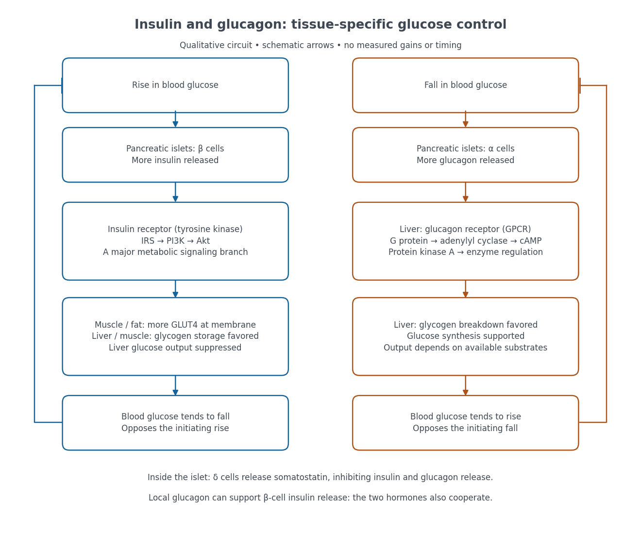
Binding to the insulin receptor, a receptor tyrosine kinase, starts phosphorylation of the receptor and insulin receptor substrates. Recruitment of phosphoinositide 3-kinase and activation of Akt transmit a major metabolic branch. In skeletal muscle and adipose tissue, that branch helps move GLUT4 to the cell membrane, increasing glucose uptake by facilitated diffusion. GLUT4 is a membrane transport protein, not an insulin receptor. Insulin also favors glycogenesis in skeletal muscle and the liver, and inhibits lipolysis in adipose tissue. In the liver, suppression of glucose output involves enzyme regulation, gene expression, and indirect changes in substrate supply. Its relative direct and indirect contributions are more complex than a single Akt arrow. [ref]
Insulin is not a universal permission slip for glucose entry: red blood cells and much of the nervous system use uptake mechanisms that are not acutely dependent on insulin. Nor does the liver use the same GLUT4 switch as skeletal muscle. This is why reduced insulin action can change blood glucose dramatically without stopping all glucose uptake. [ref]
Diabetes can disrupt production, response, and counterregulation. Type 1 diabetes usually involves destruction of beta cells and severe loss of endogenous insulin; type 2 diabetes combines insulin resistance with insufficient beta cell compensation. High circulating insulin can therefore coexist with impaired insulin action. Inappropriate glucagon release can add to excessive liver glucose output, and the response to low blood glucose can also be impaired: "more glucagon" is not a complete description of diabetes. These distinctions explain mechanisms, rather than prescribe treatment. [ref] [ref]
The motivating question was experimental: how could one recover the order in a protein when breaking all its peptide bonds destroys that order? Frederick Sanger and colleagues used complementary tests on portions of insulin. The following is an explanation of their evidence, not a laboratory recipe.
First, mark ends before destroying the chains. Sanger used the colored reagent fluorodinitrobenzene, abbreviated FDNB, to label free amino groups. After acid hydrolysis, the attached label remained on the end-residue products. Separating these derivatives by their different movement through solvents and comparing them with reference derivatives made the labels readable. The N-terminus products identified glycine and phenylalanine. Sanger emphasized that finding a stable label and a way to separate its products were both essential. See Sanger, Citation Classic (1985), discussing The free amino groups of insulin (1945). FDNB also labels suitable free amino groups on amino acid side chains, so a labeled product is not automatically an N-terminus product. See Sanger, The Chemistry of Insulin, Nobel lecture (1958), pp. 546–547.
Next, separate chains and preserve local order. Oxidation with performic acid broke the protein disulfide bonds, allowing A and B chains to be isolated. Partial hydrolysis and enzyme treatments produced fragments; these were separated and their composition and local sequences characterized. Overlaps between different fragment sets linked smaller sequences into longer ones. Many more fragments than minimally necessary were checked for consistency. See Sanger's authored Nobel lecture, pp. 547–552: chain separation, fragment analysis and sequence reconstruction.
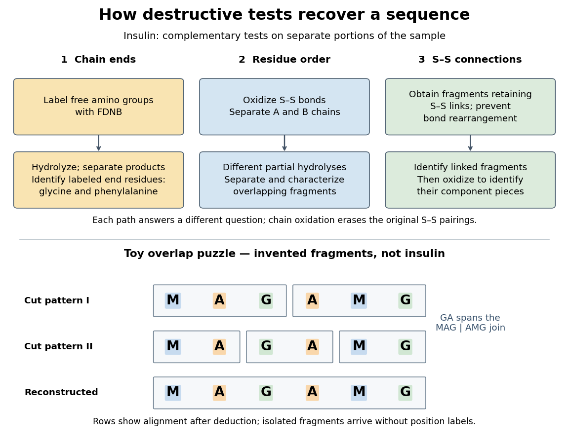
The toy fragments make the logic visible. Suppose one cut pattern yields MAG and AMG, and another yields MA, GA and MG. The first set alone permits MAGAMG or AMGMAG. The fragment GA in the second set crosses the MAG–AMG boundary in MAGAMG; it does not occur in AMGMAG. Among concatenations of the first set, therefore, the second set selects MAGAMG. This example assumes intact, correctly identified fragments from one homogeneous chain and known fragment membership in each cut pattern. Repeated stretches, missing fragments or sample mixtures can leave ambiguities; the picture illustrates inference from overlaps, not a universal guarantee of reconstruction.
Finally, determine the protein disulfide bonds separately. Oxidation used to separate whole chains erases their original connections. Sanger and colleagues instead studied fragments still joined by protein disulfide bonds, then oxidized the isolated joined fragments to identify their component pieces and locate the connected chain regions. An important trap was rearrangement of disulfide bonds during treatment: products can acquire connections absent from the starting protein. Their work therefore had to establish conditions that prevented rearrangement before interpreting a linked fragment as evidence. See Ryle and Sanger, A Disulphide Interchange Reaction, Nature 171, 1025–1026 (1953) and Sanger's Nobel lecture, pp. 553–554: preserving and identifying disulfide connections. The result was an experimentally constrained chemical structure rather than a composition list or a photograph of a fold.
The amino acid composition lists amounts or proportions of the different amino acid residues in a protein or specified polypeptide chain, without giving their order. The toy MAGAMG and MMAAGG each have counts M:2, A:2, G:2, or a proportion of each. Knowing composition therefore does not supply protein primary structure. Sanger's account begins by distinguishing the already available composition measurements from the largely unknown residue order. See Sanger's authored 1985 account of the move from composition to terminal-residue analysis.
An SH2 domain is a protein domain that recognizes a phosphotyrosine residue together with surrounding sequence features. This selective binding recruits a protein to a modified receptor or docking protein; it does not itself imply catalysis.[ref]
Signaling through Enzyme-Linked Cell-Surface Receptors. “Phosphorylated Tyrosines Serve as Docking Sites For Proteins With SH2 Domains”, Figure 15-53
The critical path method calculates an earliest schedule, a latest schedule for a chosen finish time, and each activity's task float. A critical path is a start-to-finish graph path whose total duration is greatest. There can be several such graph paths, and every one constrains completion. In the six-activity project scheduling example, the critical graph path is A-C-D-F, of duration .
Add a zero-duration source before every initial activity and a zero-duration sink after every terminal activity. Give each edge weight , including zero weight on edges leaving . This produces a weighted graph in which a graph path's weight counts every activity on it exactly once. The possible source-to-sink graph paths in our example, omitting the dummy endpoints, are A-B-D-F with weight 8, A-C-D-F with weight 10, and E-F with weight 4.
Every feasible schedule must accommodate each of these sequential chains. Consequently,This bound applies to all source-to-sink graph paths, not just the one we happen to inspect. The critical path method attains the bound by setting each activity's earliest start to the maximum of its predecessors' earliest finish times:Evaluate this recurrence in a topological order, obtained by topological sorting. Each satisfies every incoming optimization constraint, so these times form a feasible solution. The same recurrence calculates the greatest weight of a graph path from to ; hence the feasible finish matches the lower bound. This is dynamic programming on a directed acyclic graph, rather than an enumeration of all graph paths. See Paul Johnson, Scheduling and longest paths, longest-path algorithm. The linear programming formulation and its certificate are developed in project scheduling duality and unit-flow certificate for project duration.
For our project scheduling example, , , and the two merges giveF finishes at 10. All six activities are completed, even though E is absent from the critical graph path. Recording which predecessor attains each maximum lets us trace a critical graph path backward from the sink; retaining tied choices exposes multiple critical graph paths.
Now fix the project start at zero and the finish at . The latest starts come from a backward pass in reverse topological order:Every activity must finish by the earliest of its successors' latest starts, explaining the minimum here. This gives , , , , , and . These latest times themselves form a feasible solution finishing at 10. The backward calculation depends on the chosen finish time; a later deadline would give different latest times and task floats. The forward and backward passes are described in Olivier de Weck, MIT ESD.36 Lecture 2, slides 22–29.
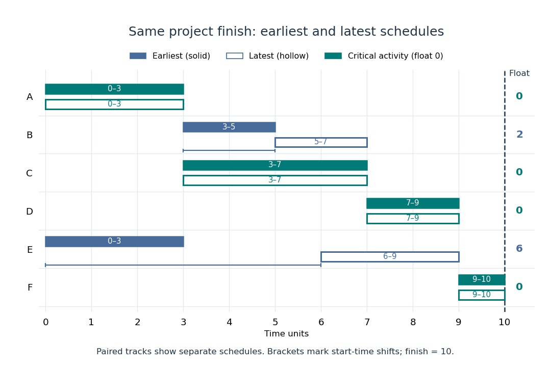
Earliest solid and latest hollow activity bars for the critical path method, with task floats of 2 for B and 6 for E
. Details. Changing a duration can change which graph paths are critical. If B's duration becomes 4, A-B-D-F and A-C-D-F both take 10: there are two critical graph paths. Shortening C alone then cannot reduce the finish time, because the chain through B still takes 10. If B's duration instead becomes 5, the earliest starts of D and F become 8 and 10, and the finish becomes 11. A-B-D-F is now the unique critical graph path; C has task float 1 relative to that new optimal finish. These calculations show why the critical path method is useful for understanding where a duration change matters, even in a project containing many parallel activities.
The syntactic priority that resolves grouping when different operators occur together without parentheses. It determines the abstract syntax tree shape before evaluation.
An arbitrary product of compact spaces is compact in the product topology. The theorem is equivalent to the axiom of choice.
The diagonal map sends to . It is an embedding of a topological space onto its diagonal subset, because either coordinate projection is its inverse on the image. For a closed oriented manifold, that subset has a fundamental class, whose Poincare dual is the cohomology class of the diagonal.
A function on a Cartesian product is a cylinder function if it depends on only finitely many coordinates. With finite discrete coordinate spaces it is a continuous function in the product topology. These functions determine finite-dimensional laws and provide a natural domain for local generators of interacting particle systems.
For a topological space and topological spaces , a function is continuous into the product topology exactly when every coordinate function is continuous.[ref]
18.901, Fall 2024 lecture notes. Lecture 5, Proposition 5.3.2, printed page 21: continuity into a product is equivalent to continuity of all component functions
Proof outline: one direction uses function composition with the continuous projection maps. For the other, the preimage of a basic cylinder set isa finite set intersection of open sets in . This gives continuity on every basic test. It explains, for example, why from the real line to is continuous in the product topology: each coordinate is a polynomial function. The general coordinate criterion fails for the box topology, where infinitely many preimages can be required at once. For example, has continuous coordinate functions, but the preimage of the box is , which is not an open set in the real line.
The box topology on has a basis of a topology consisting of all Cartesian products with every an open set in ; infinitely many coordinates may be restricted. It contains the product topology and agrees with it for finite .[ref]
18.901, Fall 2024 lecture notes. Lecture 12, Exercise 12.1.2(1)-(2), printed page 43: box basis, comparison with the product topology, and finite-factor equality
For copies of the usual real line, the box topology is strictly finer when . The box is not an open set in the product topology: a basic cylinder set containing zero leaves some coordinate unrestricted, so it contains . This is a construction for every finite coordinate set, not evidence from testing a finite prefix.
For arbitrary topological spaces , an index set , a sequence , and a point in that Cartesian product, convergence in a product space to in the product topology is equivalent to coordinatewise convergence in every factor. No countability or Hausdorff assumption on the factors is needed. For a product space of copies of the real line, regarding each point as a function identifies this with pointwise convergence.
Proof outline: the forward implication follows because each projection map is continuous. Conversely, given a basic neighborhood of , each of its finitely many coordinate tests holds for all . Taking makes all tests hold simultaneously; if is empty, any threshold works. This proves eventual membership in every neighborhood, rather than only in a sampled collection of cylinders. The same equivalence holds for nets: a directed set supplies a common upper bound for finitely many thresholds. Sequences alone need not characterize the whole topology of an arbitrary product space.
Pinned article: Introduction to the OurBigBook Project
Welcome to the OurBigBook Project! Our goal is to create the perfect publishing platform for STEM subjects, and get university-level students to write the best free STEM tutorials ever.
Everyone is welcome to create an account and play with the site: ourbigbook.com/go/register. We belive that students themselves can write amazing tutorials, but teachers are welcome too. You can write about anything you want, it doesn't have to be STEM or even educational. Silly test content is very welcome and you won't be penalized in any way. Just keep it legal!
Intro to OurBigBook
. Source. We have two killer features:
- topics: topics group articles by different users with the same title, e.g. here is the topic for the "Fundamental Theorem of Calculus" ourbigbook.com/go/topic/fundamental-theorem-of-calculusArticles of different users are sorted by upvote within each article page. This feature is a bit like:
- a Wikipedia where each user can have their own version of each article
- a Q&A website like Stack Overflow, where multiple people can give their views on a given topic, and the best ones are sorted by upvote. Except you don't need to wait for someone to ask first, and any topic goes, no matter how narrow or broad
This feature makes it possible for readers to find better explanations of any topic created by other writers. And it allows writers to create an explanation in a place that readers might actually find it.
Figure 1. Screenshot of the "Derivative" topic page. View it live at: ourbigbook.com/go/topic/derivativeVideo 2. OurBigBook Web topics demo. Source. - local editing: you can store all your personal knowledge base content locally in a plaintext markup format that can be edited locally and published either:This way you can be sure that even if OurBigBook.com were to go down one day (which we have no plans to do as it is quite cheap to host!), your content will still be perfectly readable as a static site.
- to OurBigBook.com to get awesome multi-user features like topics and likes
- as HTML files to a static website, which you can host yourself for free on many external providers like GitHub Pages, and remain in full control

Figure 2. You can publish local OurBigBook lightweight markup files to either OurBigBook.com or as a static website.
Figure 3. Visual Studio Code extension installation.
Figure 5. . You can also edit articles on the Web editor without installing anything locally. Video 3. Edit locally and publish demo. Source. This shows editing OurBigBook Markup and publishing it using the Visual Studio Code extension. 
- Infinitely deep tables of contents:




All our software is open source and hosted at: github.com/ourbigbook/ourbigbook
Further documentation can be found at: docs.ourbigbook.com
Feel free to reach our to us for any help or suggestions: docs.ourbigbook.com/#contact