Topics (384k) Articles (398k) Users (410) Discussions (242) Comments (383) Files (13k) New article
A speckle pattern is a granular intensity pattern from coherent wave interference. In stellar imaging, residual wavefront errors produce speckles around the central point spread function.
A point spread function is an imaging system's response to an optical point source. Here it means the distribution of image light intensity: an ideal point object becomes a finite spot, often with faint rings, because of diffraction. An unresolved star and a sufficiently small bead emitting fluorescence are practical approximations to an optical point source. Their image tells us how nearby object details will overlap, and reveals blurring from optical aberrations, defocus, and, for an optical telescope, astronomical seeing.
A useful convention separates shape from throughput. At a fixed image plane, let be the point spread function with . Its units are inverse area. A point delivering detected radiant flux at image position produces light intensity ; this point spread function normalization makes the integral over the image equal to . A profile divided by its own peak is convenient for comparing widths, but is a different point spread function normalization and does not by itself compare total radiant flux.
In incoherent imaging, different object points have negligible mutual spatial optical coherence over the measurement, so their image light intensities add. If the response also obeys translation invariance over the chosen field of view, the expected continuous image is the convolutionHere is the object brightness distribution expressed in image-scaled coordinates, with magnification already included, and is constant transmission. For , where is the two-dimensional Dirac delta function, this gives . A changing response across the field of view instead requires a position-dependent integral kernel ; one measured point spread function is then only a local calibration.
In coherent imaging, the superposition principle applies to the complex wave amplitudes. With amplitude spread function , the corresponding ideal model isThus generally differs from : coherent contributions produce wave interference terms that depend on their relative wave phases. Their time average vanishes for mutually incoherent emitters, which explains the intensity convolution. Partial optical coherence requires the correlations between object points as well.[ref]
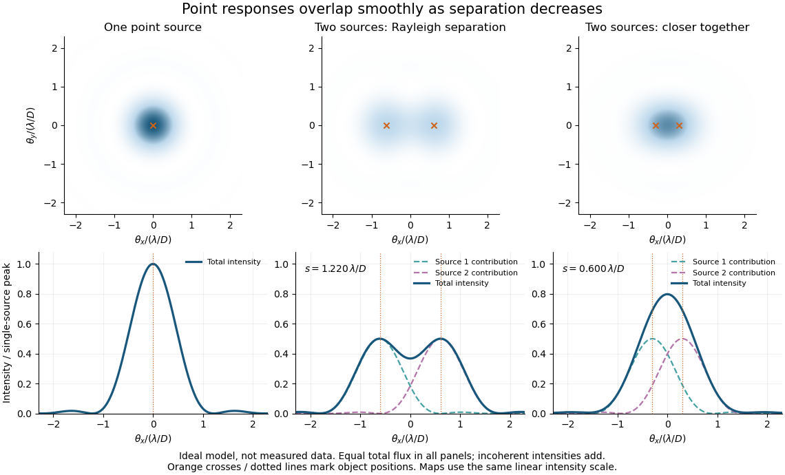
Ideal circular-pupil point responses and the overlap of two mutually incoherent sources
. Details. The figure is an original diffraction model, not measured data. All panels have the same total radiant flux: each member of a pair contributes half the single-source radiant flux. Dashed curves show the separate light intensity contributions; the solid curve is their sum. The point spread functions have tails, so even sources satisfying the Rayleigh criterion overlap. As separation decreases, the image changes continuously; there is no abrupt disappearance of all information at one separation.
A motivating measured example is Measurement of point-spread function (PSF) for confocal fluorescence microscopy by InCheon Song and others (2005). A laser, delivered through an optical fiber, excited fluorescent beads on a slide through a , numerical aperture oil-immersion objective. A moving stage scanned the bead; emitted light returned through the objective, an emission filter and a pinhole to a photodiode. The readout was fluorescence light intensity against scanned position. Under the same setup, nominal bead diameters , , and produced progressively broader measured spots. The size comparison controls for the finite object: the measured response is the convolution of bead emission with the effective point spread function, rather than a pure point response. Inverting this convolution model gave a response compared with the theoretical one. The smaller bead gave a weaker signal relative to noise; uncertainty in actual bead diameter also affected the restored width. These are limits of the calibration. In confocal microscopy, excitation and pinhole detection jointly determine the effective point spread function; this experiment does not measure the ideal widefield Airy disk plotted above.[ref]
For a new calibration, useful additional controls are to measure detector background, avoid saturating the photodetector, repeat the scan to check stability, and compare isolated beads at several positions in the field of view. Record wavelength, numerical aperture, pinhole setting, sampling interval and optical focus. These are practical recommendations, not extra measurements claimed for the published experiment.
The free spectral range is the wavelength or frequency spacing between adjacent orders or resonances of an optical instrument. It identifies when different orders can overlap. Always specify the coordinate: a uniform spacing in frequency need not be uniform in wavelength. For an ideal Fabry–Pérot interferometer at normal incidence, with mirror separation and constant refractive index , Fabry–Pérot resonance spacing gives , where is the speed of light in vacuum. The free spectral range of an echelle grating follows a different order condition.
A diffraction grating is a periodic optical structure whose repeated slits or grooves direct light into diffraction orders through wave interference. Its beauty is that many individually broad contributions cooperate to select narrow directions: the spacing determines where the principal peaks occur, while the number of illuminated elements determines how sharply they are selected. This makes a diffraction grating useful in a spectrometer, where separating wavelengths spatially lets us examine an optical spectrum. [ref]
https://ocw.mit.edu/courses/6-007-electromagnetic-energy-from-motors-to-lasers-spring-2011/4835d62777f42e82a40c319defcc80a6_MIT6_007S11_lec28.pdf. MIT 6.007: Multiple-slit diffraction and spectrometer application, slides 5-6
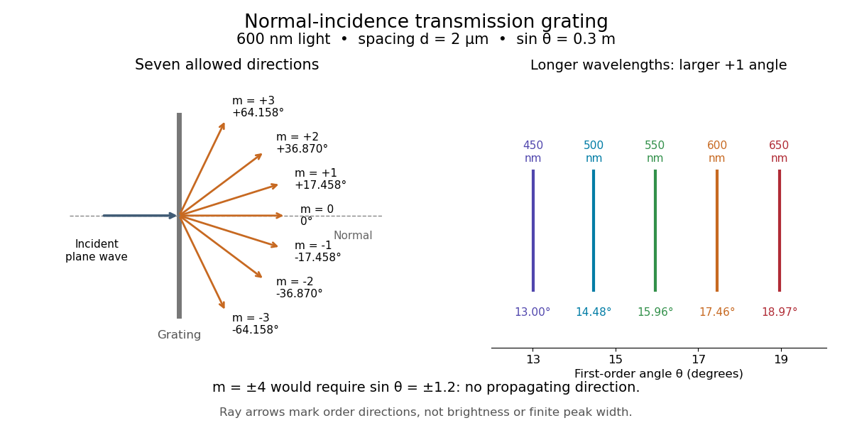
.Consider a transmission diffraction grating in air, illuminated at normal incidence by a plane wave. Let be the centre-to-centre slit spacing, the wavelength in the surrounding medium, and the signed outgoing angle from the forward normal. In Fraunhofer diffraction, where observation directions specify the far-field pattern, adjacent contributions have path difference and phase difference . Their wave amplitudes reinforce whenever , giving . This normal-incidence geometry should be kept distinct from the incident and reflected angle convention in the grating equation below. [ref].
Angular colour separation follows immediately. At fixed nonzero diffraction order, increasing the wavelength moves the peak farther from the normal. With , first-order light at leaves at , whereas leaves at : a separation of . The zero diffraction order stays at for both wavelengths. Thus grating dispersion comes from an orderly dependence of wave interference on wavelength, rather than an arbitrary assignment of colours to directions.
For identical slits with uniform coherent illumination, meaning stable relative wave phases across the array, the normalized wave interference factor isThe apparent at a principal peak has limiting value one. A short explanation uses the geometric series: equal wave phases add equal complex amplitudes; a small directional change distributes those contributions around the complex plane and allows cancellation. With each slit's contribution held fixed, peak scalar wave intensity scales as . The normalized plots remove that height change to make the narrowing visible. Stable relative wave phases, or optical coherence, are essential; a sum of independent intensities would lose this array structure. [ref]
https://farside.ph.utexas.edu/teaching/315/Waveshtml/node93.html. Richard Fitzpatrick, University of Texas: Multi-slit interference, equations 10.38-10.40
.For finite slit width , the ideal rectangular-slit model multiplies by a broad single-slit diffraction envelope:The sinc function factor, extended continuously at , controls the brightness available to the narrow peaks. For example, gives envelope values about , , and at diffraction orders , , and in the example. If an envelope zero coincides with an allowed diffraction order, that peak disappears. A permitted direction therefore need not produce a visible bright spot. [ref]
https://www.mit.edu/course/other/viz/EM/visualizations/notes/modules/guide14.pdf. MIT: Single-slit envelope and absent interference maxima, sections 14.6-14.7
.Historically, Joseph von Fraunhofer used fine parallel wires stretched between threaded rods to make diffraction gratings. Kenyon's historical apparatus account describes both this construction and a later reconstruction with visible light. The example makes the governing idea tangible: regular spacing can turn a simple array of obstacles into an instrument for distinguishing wavelengths. [ref]
https://physics.kenyon.edu/EarlyApparatus/Optics/Diffraction_Grating/Diffraction_Grating.html. Thomas B. Greenslade Jr., Kenyon College: Diffraction grating
.Wave interference is the reinforcement or cancellation that occurs when overlapping wave amplitudes add by the superposition principle. For two monochromatic waves of the same frequency, mutual optical coherence means that their relative wave phase is stable during the observation. Equal wave phases give constructive interference; a half-cycle phase difference gives the destructive interference intensity minimum. Wave amplitudes add before their squares determine wave intensity. [ref]
https://openstax.org/books/university-physics-volume-3/pages/3-1-youngs-double-slit-interference. Ling, Sanny and Moebs, University Physics Volume 3, §3.1: coherent waves and interference
.Consider two overlapping beams in a homogeneous medium, with the same polarization of an electromagnetic wave and individual local time-averaged light intensities . Their phase difference is measured in radians. In the scalar detection convention, the combined local time-averaged wave intensity isThe last term records wave interference; adding alone misses it. The formula describes irradiance when both fields propagate along the same direction, or when the same detector geometry factor is included in all three intensities. For crossing beams it describes the squared electric field response, proportional to scalar wave intensity; a specified component of the Poynting vector also requires the propagation geometry. The ideal crossing plane waves below make that distinction explicit.
For equal individual light intensities , the cosine half-angle identity givesThe constructive interference intensity is at modulo , and the destructive interference intensity is zero at modulo . At phase quadrature, , it is . With and in the same arbitrary wave intensity unit, the maximum is , the minimum is , and the phase quadrature value is : unequal wave amplitudes cannot cancel completely.
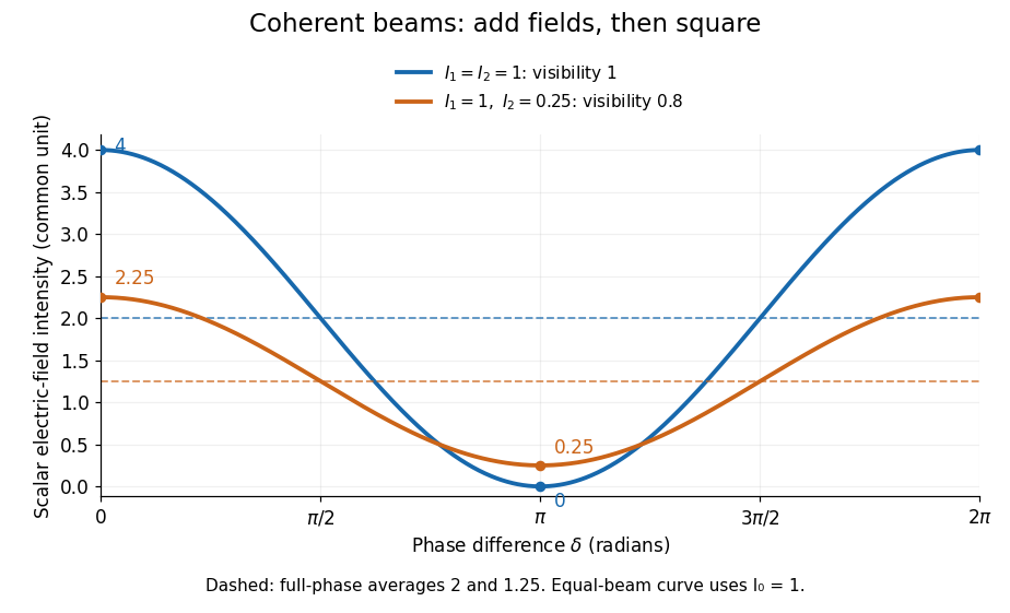
Two-beam wave intensity versus phase difference: equal beams reach 4 and 0; unequal beams reach 2.25 and 0.25
. Details. Both curves use the same wave intensity unit and a horizontal angle in radians. The dashed levels are the averages over a full phase difference cycle. Equal beams have interferometric visibility one; the unequal example has interferometric visibility .
A spatially varying phase difference turns the same law into interference fringes. Take two ideal plane electromagnetic waves with common wavelength , equal individual light intensities , and propagation directions at angles and from the axis in the plane, with . Both have linear polarization along , perpendicular to both propagation directions. Choose equal initial wave phases; their wavevectors and phase difference areHere is the wavenumber and the angular frequency. The common and time terms cancel, so the interference fringes stay at fixed for every . Their interference fringe spacing isSet the length unit to , so that , and take : then . The constructive interference intensity bands lie at integer ; the destructive interference intensity bands lie at half-integer .
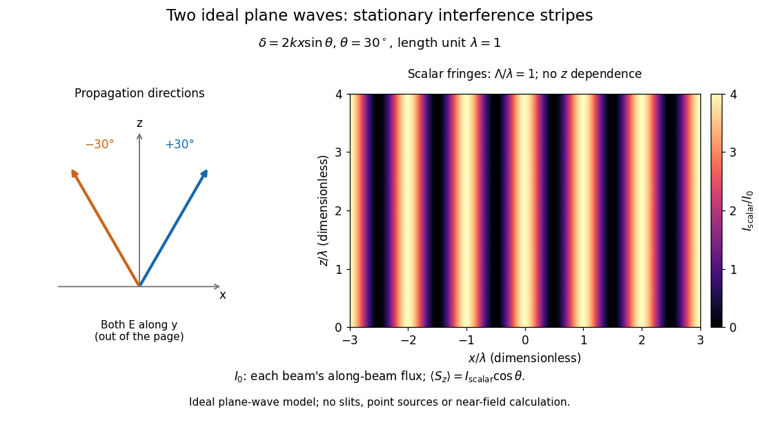
The grid covers and ; both axes are dimensionless lengths in wavelength units. The colour scale is from zero to four, using the same single-beam normalization as the equal-beam curve above. This is an ideal plane wave superposition, with no slits or point sources and no near-field approximation. For these -polarized plane electromagnetic waves in vacuum, the longitudinal time-averaged Poynting vector obeys ; the plotted scalar therefore differs from the irradiance through a plane normal to by that common factor. This relation follows by adding the magnetic fields as well as the electric fields.
The bright peaks do not create energy. Averaging over one interference fringe spacing, or equivalently over one full phase difference cycle, givesbecause the integral of the cosine is zero, with sine as its antiderivative. Equal beams thus average to , despite bright bands at . For the crossing-wave geometry, the average longitudinal energy flux is correspondingly . Bright and dark regions redistribute the incoming energy; conservation of energy concerns the full energy flux, rather than the height of one peak.
Wave interference is useful because phase differences convert small changes in optical path length into measurable changes of wave intensity, as in a Mach-Zehnder interferometer. Its beauty is that the same superposition principle produces both complete cancellation and fourfold brightening; adding more coherent contributions also produces the narrow peaks of a diffraction grating. Feynman's treatment connects this many-source pattern directly to addition of complex amplitudes. [ref].
A short proof outline uses local real fields with parallel linear polarizations. Write and for the same positive conversion factor . Averaging over many wave periods while the phase difference stays fixed uses and , giving the stated law. Equivalently, add the complex amplitudes and take the squared complex modulus. [ref]
https://www.feynmanlectures.caltech.edu/I_29.html#Ch29-S5. Feynman, Leighton and Sands, The Feynman Lectures on Physics, I §29–5: the mathematics of interference
.For different fixed linear polarizations in a common transverse plane, the cross term acquires the dot product of their real unit vectors, equal to for relative angle . Orthogonal linear polarizations remove the cross term in polarization-insensitive scalar detection; different orientations generally only reduce it. A common polarizer can select overlapping components and recover wave interference. Likewise, rapid random variation of the phase difference removes the observed cross term only when the detector's time average has . Slowly varying wave phases can instead move resolved interference fringes, and biased or incompletely sampled wave phases can leave residual contrast. Finite optical coherence therefore depends on the observation time as well as the fields.
A wavefront connects points with the same wave phase at one specified time. It is a surface, rather than the trajectory of a particular piece of light. For a scalar monochromatic wave written as , a wavefront is a connected level set of the phase function ; different surfaces can share the same wave phase modulo . A plane wave has planar wavefronts. An outward wave from an ideal point source in a uniform medium has spheres as wavefronts, while an optical lens can turn nearly planar wavefronts into converging ones. The wavefront describes wave phase, not wave amplitude: drawing it does not say how bright the beam is. [ref]
The relation to light rays becomes precise in a stationary medium with isotropy, negligible loss and a real positive scalar refractive index . In the geometrical optics limit, spatial changes in the refractive index and wave amplitude are slow on the local wavelength scale. For a single smooth propagation branch, writeHere is the angular frequency, is the vacuum speed of light, has units of length, and the last relation is the optical eikonal equation. The local wavevector is . Its direction is normal to a smooth wavefront, since a gradient is normal to its level sets. A forward light ray has unit tangent vector , so it follows this normal under the stated assumptions. Along that light ray, : the change in is the optical path length. This is the short geometric argument linking wavefronts, light rays and optical path length. [ref]
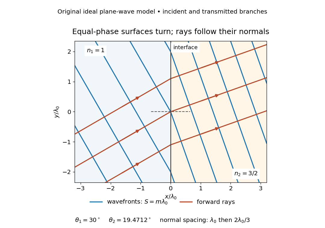
The diagram shows incident and transmitted branches separately, with the reflected branch omitted. Its stipulated refractive indices are and , and its incident angle is to the interface normal. At a stationary interface, the frequency and tangential wavevector agree on the two sides: Snell's law gives , hence . The wavefronts turn while their normal spacing decreases from to , where is the vacuum wavelength. More explicitly, with normal to the interface and tangential, take for and for . These functions agree at ; the drawn wavefronts are at with . This is an exact piecewise plane wave phase construction for the stipulated transparent media, not measured material data. [ref]
The normal-to-wavefront rule requires its assumptions. In a medium with anisotropy, the wavevector remains normal to a smooth wavefront, but the group velocity and energy flux need not follow it. [ref] Near a wave caustic, where multiple light rays meet, one smooth phase function may no longer describe the field; diffraction and the full wave amplitude matter. A wavefront is also not generally a surface of equal pulse arrival time. In a medium with optical dispersion, a monochromatic wave phase moves with the phase velocity, while a sufficiently narrow wave packet follows the group velocity. Even identical optical path lengths at one frequency can give different group delays. The usual equal-travel-time picture needs a common launch reference and a nondispersive ray model; an arbitrary broadband disturbance has no single monochromatic wavefront.[ref]
Phase conjugation creates a returning monochromatic wave whose spatial complex amplitude is proportional to the complex conjugate of the incident field. Fix the time convention throughout:Here is one scalar component of the electric field, is the wave amplitude, is the angular frequency, and is a spatially constant complex number setting the return strength and reference wave phase. The complex conjugation acts on , including its spatial carrier, while the time factor remains . Conjugating both factors would merely give another representation of the same real field. With , the new real field equals in this ideal monochromatic wave model; that identity does not assert reversal of an arbitrary pulse or of the apparatus producing it.
The spatial wave phase becomes , so the local wavevector changes from to . For example, with becomes : both components of the wavevector reverse. In a transparent stationary medium with isotropy and positive refractive index, light rays follow the wavevector, giving counterpropagation. The same wavefronts now have opposite propagation normals. This is why phase conjugation can return a distorted beam toward its origin: it reverses the detailed spatial wave phase, rather than requiring that wave phase to be flat.
The attractive application is correction of optical aberrations accumulated on an outward trip. The return uses the distortion itself as the prescription for correction, as the original thin phase-plate cancellation by phase conjugation example makes explicit. An experimentally accessible implementation measures the spatial wave phase and uses a spatial light modulator to generate its negative; digital optical phase conjugation describes an inspected 2010 demonstration of recovery through multiple scattering.
A fundamental Gaussian beam is an ideal beam of light whose transverse wave amplitude has a Gaussian function profile. Here consider a circularly symmetric beam in vacuum, with propagation along , two transverse coordinates , and radius from the optical axis. With the beam waist at , total power , and vacuum wavelength , its time-averaged light intensity, meaning irradiance in , isHere is the minimum beam radius, and is the Rayleigh range. Far from the beam waist, with beam divergence half-angle . These are the fundamental circular Gaussian beam laws within the scalar paraxial approximation, appropriate when and the beam divergence is small. The underlying envelope solves the parabolic wave equation exactly; this does not make it an exact vector solution of Maxwell equations. [ref].
The radius convention matters. Writing for the complex wave amplitude envelope, the same is the wave amplitude radius and the light intensity radius:At these ratios are and , respectively. The light intensity radius is instead . None of these radii is a sharp edge: the ideal Gaussian function has nonzero tails at every finite radius. Kogelnik and Li explicitly use the wave amplitude radius in their fundamental-mode treatment. [ref]
https://dielslab.unm.edu/sites/default/files/Kogelnik66_0.pdf. Herwig Kogelnik and Tingye Li, Laser Beams and Resonators, Applied Optics 5, 1550–1567, 1966, §3.2
.For a numerical example, take vacuum wavelength and beam waist radius . Substitution gives Rayleigh range and far-field beam divergence half-angle . At , the beam radius is and the on-axis irradiance is half its waist value. At the same wavelength, halving the beam waist radius to quarters the Rayleigh range to and doubles the beam divergence half-angle to . At fixed power, that smaller beam waist also quadruples the peak irradiance.
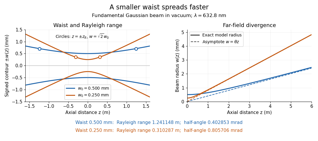
Gaussian beam radii at 632.8 nm: a smaller beam waist gives a shorter Rayleigh range and greater beam divergence
. Details. The contours in the left panel are in a plane through the optical axis; they mark an light intensity level, not an outer boundary. The right panel compares the exact model radii with the far-field asymptotes . The horizontal and vertical axes use different length units, so the drawn slopes are not physical angles.
The normalization expresses conserved power during free propagation. In transverse polar coordinates, an annulus has area , soA proof outline is the substitution in this integral. Spreading reduces peak irradiance as while increasing transverse area as , leaving power unchanged. In particular, the disk of radius contains , or , of the total power; the local light intensity at its rim is only of the on-axis light intensity. These are different quantities.
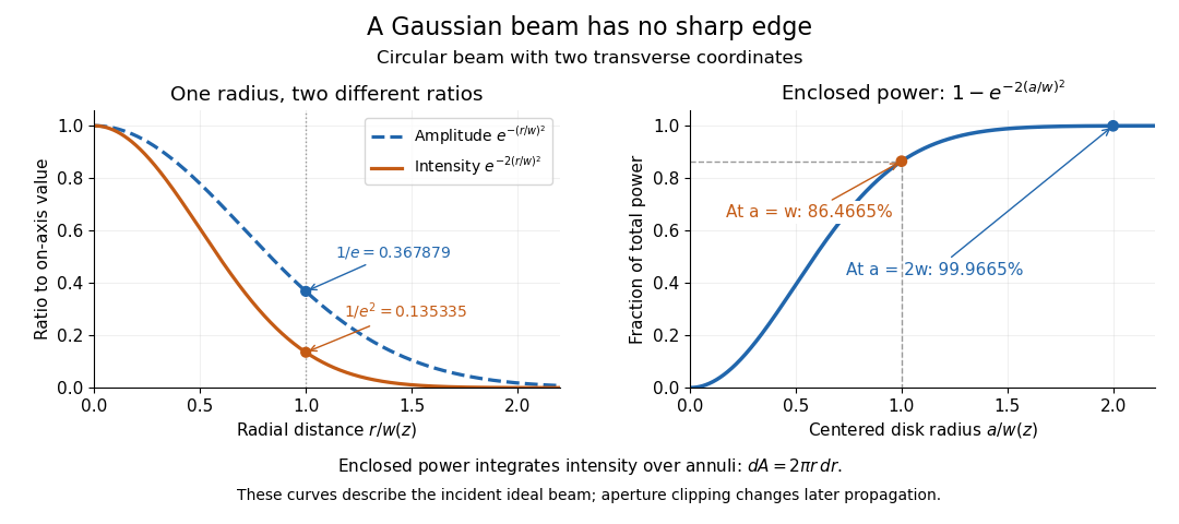
The left panel compares normalized wave amplitude magnitude and irradiance; the right panel integrates the transverse area to show enclosed power. For an ideal absorbing circular aperture of radius centered on the optical axis, the same fraction gives the power passing the aperture at that plane. An aperture of radius clips about of the incident power; radius clips only , or . After clipping, extra diffraction means the transmitted field no longer obeys the unmodified ideal Gaussian beam law. Every finite aperture cuts some ideal tail. Kogelnik and Li distinguish their large-aperture beam analysis from their finite-aperture diffraction analysis. [ref]
https://dielslab.unm.edu/sites/default/files/Kogelnik66_0.pdf. Kogelnik and Li, 1966, §§3–4
.The useful tradeoff is that a small bright spot cannot remain narrow indefinitely. An optical lens can create a smaller beam waist, but diffraction then makes the beam spread faster. The particularly simple relation ties localization directly to beam divergence. A proof outline for the propagation law starts with . The parabolic wave equation separates into two transverse factors, and a Gaussian integral in each coordinate givesHere is dimensionless and is the wavenumber; the carrier convention is , with angular frequency . Taking the squared complex modulus gives the stated and its light intensity scaling. Each transverse factor contributes , explaining the prefactor here and the different prefactor in the preserved Gaussian beam with one transverse coordinate.
Historically, Gaussian beam theory developed alongside early laser resonator theory and lens-guided transmission. In their 1966 review, Kogelnik and Li credit Boyd and Gordon, and Goubau and Schwering, with early beam treatments; they summarize earlier work rather than claim the whole construction as a new discovery. Their paper brings beam propagation, focusing and finite-aperture diffraction into a common practical account. [ref]
https://dielslab.unm.edu/sites/default/files/Kogelnik66_0.pdf. Kogelnik and Li, 1966, introduction and §3
.For a planar autonomous differential equation , , an -nullcline is a set where and a -nullcline is a set where . Their intersections are equilibrium points. Away from intersections, the vector field is vertical on an -nullcline and horizontal on a -nullcline.
For , , the nullclines are and . On the vertical velocity is , and on the horizontal velocity is . Signs in the four intervening sectors complete a qualitative phase portrait.
For a permutation of , an inversion is a pair with . Its number equals the Coxeter length for adjacent transpositions: each adjacent swap changes the count by one, and swapping adjacent descents sorts the permutation in exactly that many steps.
A limit cycle is an isolated periodic orbit of a dynamical system. It is attracting if nearby orbits approach it in forward time. A continuous family of closed orbits around a center equilibrium does not consist of limit cycles, because its members are not isolated.
A thermal path integral represents the canonical partition function by paths periodic in Euclidean time of circumference . For , its formal action is . The periodic boundary condition results from taking the trace of the evolution kernel. The continuum measure requires a regularization and normalization; finite-dimensional measures make both choices explicit.
For a countable set , join two points outside through an auxiliary point avoiding the countably many lines through either endpoint and a point of . Such an auxiliary point exists: choose a line with direction outside the countable list of forbidden directions, then avoid its countably many intersections with those lines. The two segments avoid , giving a continuous path.
A heated particle suspension can have competing compositional and thermal contributions to its mass density. Let be the carrier-fluid mass density at reference temperature , the particle mass density and the carrier-fluid thermal expansion coefficient. In a dilute mixture, neglecting products of small changes,where is particle volume fraction, and . Heavy particles increase mass density, whereas warming an ordinarily expanding carrier fluid decreases it.
For a well-mixed layer of fixed depth with an absorbing horizontal bed, particle deposition flux gives , if is a constant downward settling velocity magnitude and other particle fluxes vanish. A separate heat balance determines . Their different time dependences can change the sign of , reversing the layer's reduced gravity relative to fluid at the reference state. A resulting unstable density stratification can invalidate the well-mixed or one-dimensional settling assumptions, so the density balance is also a consistency check on the model.
An ill-posed problem fails existence, uniqueness or continuous dependence in the specified function spaces. Backward heat equation evolution is unstable because its Fourier modes grow like , making arbitrarily small high-frequency errors grow without a uniform bound.
The parity operator acts on a spatial wavefunction by and satisfies . For a Hamiltonian operator with an even potential and parity-invariant domain, . A nondegenerate energy eigenvalue has a one-dimensional eigenspace, so its eigenfunction is an eigenvector of with eigenvalue or .
Angular momentum of a radial function times a linear polynomial by  Codex 0 Created 2026-10-05 Updated 2026-11-05
Orbital angular momentum operators annihilate a radial multiplier . Their squared sum sends every degree-one homogeneous polynomial to times that polynomial, so a nonzero normalizable state has angular momentum quantum number . With real and real coefficients, its third-component expected value is zero by angular symmetry, though it need not be an eigenstate of that component.
For a compact topological surface with cone-point orders , the orbifold Euler characteristic is . An orbifold covering multiplies this quantity by its degree.
Given a cost and probability measures , the Monge problem minimizes over measurable transport maps with pushforward measure . The feasible set may be empty because a map cannot split an atom of a measure.
The Kantorovich problem minimizes over transport plans with marginal distributions . It relaxes the Monge optimal transport problem by allowing source mass to split among destinations.
Pinned article: Introduction to the OurBigBook Project
Welcome to the OurBigBook Project! Our goal is to create the perfect publishing platform for STEM subjects, and get university-level students to write the best free STEM tutorials ever.
Everyone is welcome to create an account and play with the site: ourbigbook.com/go/register. We belive that students themselves can write amazing tutorials, but teachers are welcome too. You can write about anything you want, it doesn't have to be STEM or even educational. Silly test content is very welcome and you won't be penalized in any way. Just keep it legal!
Intro to OurBigBook
. Source. We have two killer features:
- topics: topics group articles by different users with the same title, e.g. here is the topic for the "Fundamental Theorem of Calculus" ourbigbook.com/go/topic/fundamental-theorem-of-calculusArticles of different users are sorted by upvote within each article page. This feature is a bit like:
- a Wikipedia where each user can have their own version of each article
- a Q&A website like Stack Overflow, where multiple people can give their views on a given topic, and the best ones are sorted by upvote. Except you don't need to wait for someone to ask first, and any topic goes, no matter how narrow or broad
This feature makes it possible for readers to find better explanations of any topic created by other writers. And it allows writers to create an explanation in a place that readers might actually find it.
Figure 1. Screenshot of the "Derivative" topic page. View it live at: ourbigbook.com/go/topic/derivativeVideo 2. OurBigBook Web topics demo. Source. - local editing: you can store all your personal knowledge base content locally in a plaintext markup format that can be edited locally and published either:This way you can be sure that even if OurBigBook.com were to go down one day (which we have no plans to do as it is quite cheap to host!), your content will still be perfectly readable as a static site.
- to OurBigBook.com to get awesome multi-user features like topics and likes
- as HTML files to a static website, which you can host yourself for free on many external providers like GitHub Pages, and remain in full control

Figure 2. You can publish local OurBigBook lightweight markup files to either OurBigBook.com or as a static website.
Figure 3. Visual Studio Code extension installation.
Figure 5. . You can also edit articles on the Web editor without installing anything locally. Video 3. Edit locally and publish demo. Source. This shows editing OurBigBook Markup and publishing it using the Visual Studio Code extension. 
- Infinitely deep tables of contents:




All our software is open source and hosted at: github.com/ourbigbook/ourbigbook
Further documentation can be found at: docs.ourbigbook.com
Feel free to reach our to us for any help or suggestions: docs.ourbigbook.com/#contact