
Past exam of the mathematics course of the University of Cambridge 2005 ia Paper 3 11A Solution Created 2026-09-24 Updated 2026-10-14
At a critical point of a twice continuously differentiable real function, and the Taylor expansion isThe real symmetric Hessian matrix has an orthonormal eigenbasis, so writing gives . If every eigenvalue is positive, this quadratic form is at least , and the remainder cannot change its sign for sufficiently small nonzero . Thus is a strict local minimum. If every eigenvalue is negative, the analogous argument gives a strict local maximum. If positive and negative eigenvalues both occur, displacement along the corresponding eigenvectors gives values above and below , so is a saddle point of a scalar function.
The second-derivative test can be inconclusive when the Hessian matrix is singular and semidefinite: higher-order terms along directions in the kernel of a linear map matter. For example and have the same Hessian at zero, but the first has a strict minimum and the second a saddle point of a scalar function. A zero eigenvalue does not prevent a saddle conclusion if other eigenvalues already have both signs.
For the given function write . Its first derivatives areThe origin is a critical point for every real , withIts eigenvalues are , so it is always a saddle point of a scalar function. If one coordinate at a critical point is zero, the other must also be zero. If both are nonzero, the derivative equations force , possible only for . Hence for the origin is the only critical point.
For there are four additional critical points,At such a point,Thus the two equal-sign points are strict maxima, and the two opposite-sign points are strict minima. They are global: implieswhere the last maximum occurs at and equality also requires .
As , the four nonzero critical points have distance from the origin and escape to infinity, rather than merging with the origin. Their values diverge as . As from below there are no extra critical points, while the origin stays a saddle throughout. This is critical points escaping to infinity in a Gaussian-weighted bilinear function.
Past exam of the mathematics course of the University of Cambridge 2005 ia Paper 3 10A Solution Created 2026-09-24 Updated 2026-10-14
For an oriented piecewise smooth surface and a continuously differentiable vector field, Stokes theorem stateswhere the boundary orientation is induced by through the right-hand rule. Choose the upward orientation of the elliptic paraboloid. Its band has cylindrical radius , and a parametrization isIts oriented surface element and scalar area element areThe requested sketch shows the open band, not a capped solid.
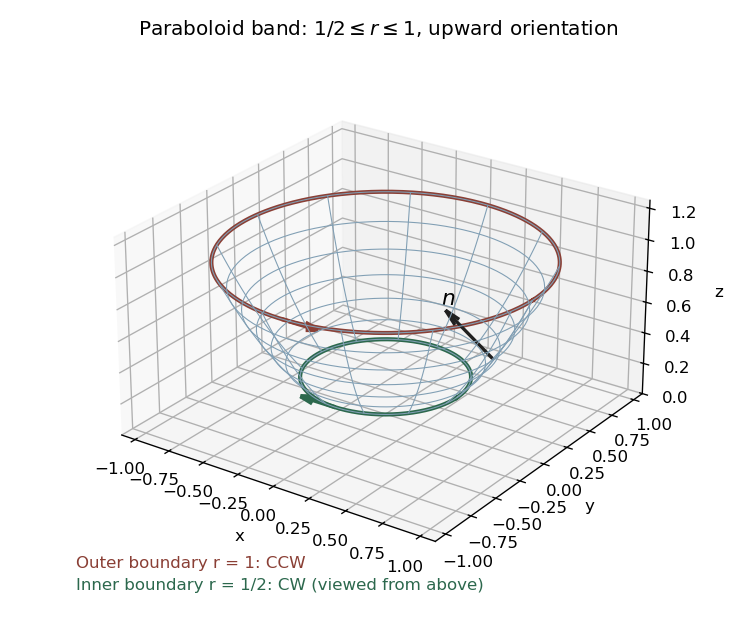
Upward-oriented annular paraboloid band, with counterclockwise outer boundary and clockwise inner boundary
. Details. 
For the specified vector field, direct differentiation gives . HenceTo check this by Stokes theorem, parametrize a counterclockwise circle of radius at height by . Along it , andUsing gives . The induced outer circle is counterclockwise as viewed from above, and the inner circle is clockwise. ThereforeThis verifies the direct surface integral and the Stokes flux through an annular paraboloid. Reversing the chosen surface orientation reverses the final sign.
Past exam of the mathematics course of the University of Cambridge 2005 ia Paper 2 9F Solution Created 2026-09-24 Updated 2026-10-14
The expectation of a complex random quantity is defined through its real and imaginary parts. Both and are bounded, so all expectations below exist. Expand the addition formulae and apply the expectation of a product of independent random variables identity:Combining real and imaginary parts provesFor the simple symmetric random walk, write , with independent increments satisfying . The usual casino model uses these independent, or conditionally fair, increments. Their characteristic function is , so repeated factorization givesThis is real for real . Equivalently, the distribution of is symmetric, making .
For any integer , Fourier orthogonality givesThe random walk has finite support, so we may interchange its finite expectation with this integral. ThereforeFor even , evenness and reflection symmetry about reduce this toFor odd , has odd parity and cannot be zero, so . As a separate combinatorial check, for the return probability is , since exactly positive increments are required.
Past exam of the mathematics course of the University of Cambridge 2005 ia Paper 2 8B Solution Created 2026-09-24 Updated 2026-10-14
On an interval where are continuous, define the WronskianUsing the two second-order linear differential equations to eliminate the second derivatives givesThe integrating factor yields the Abel identityThus the Wronskian either vanishes identically or is nonzero everywhere on the interval. If are linearly dependent, it is identically zero. Conversely, if , the two initial-data vectors are dependent, so some nontrivial linear combination has both value and first derivative zero at . The uniqueness theorem for ordinary differential equations makes that combination identically zero. Hence the solutions are linearly independent exactly when their Wronskian is nonzero at one, and therefore every, point. Continuity and the common differential equation are essential to this converse.
For the particular equation, divide by on either interval or . The coefficient of is zero, so its Wronskian is constant there. The proposed satisfies . To construct a second solution by reduction of order, imposeDividing by shows that , givingTaking producesThe nonzero Wronskian proves linear independence; hence the general solution on either nonsingular interval is . Zero is a singular point of a differential equation and is excluded from this construction.
Past exam of the mathematics course of the University of Cambridge 2005 ia Paper 2 7B Solution Created 2026-09-24 Updated 2026-10-14
For , the polar coordinates satisfyA positive constant radius must therefore be one. The nonconstant periodic solutions arewith least period and counterclockwise orientation. The origin is also a stationary solution, hence periodic in the degenerate sense of a constant function; it is a point rather than a nontrivial closed orbit. There are no other constant-radius solutions.
For , put . Then , a logistic differential equation. Solving this separable differential equation givesThe denominator is positive for every forward time. When , the radius increases monotonically to one; when , it decreases monotonically to one; and when it stays there. Thus every nonzero orbit approaches the unit circle while continuing to rotate. More precisely, its distance from the phase-matched circular solution tends to zero; its Cartesian coordinates do not converge to a single point. For , the solution stays at the origin.
The origin is the only equilibrium point. Its Jacobian matrix iswhose eigenvalues are . It is an unstable focus. The unit circle is an attracting limit cycle, rather than a curve of equilibria: on it the vector field remains nonzero. Linearizing the radial equation at gives , confirming radial attraction. All other radii are strictly monotone, so there are no additional nontrivial periodic orbits.
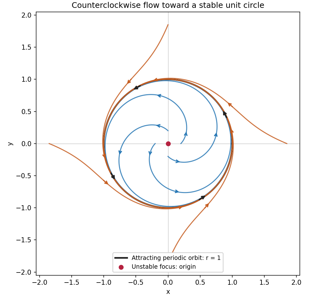
Counterclockwise spirals approach an attracting unit circle around an unstable equilibrium
. Details. 
Past exam of the mathematics course of the University of Cambridge 2005 ia Paper 2 6B Solution Created 2026-09-24 Updated 2026-10-14
Substitution of the power series, with termwise differentiation, gives the coefficient identityThus and are arbitrary, and all power series solutions of the Hermite differential equation areAn empty product is one. For a nonterminating branch the ratio of consecutive terms in its own parity subsequence is asymptotic to , hence tends to zero for every fixed . The ratio test proves convergence everywhere; the resulting power series can be differentiated termwise and indeed solve the differential equation. A terminating branch is already a polynomial.
The boundary condition forces ; the solution is odd. Apart from the zero solution, which works for every , a polynomial occurs exactly when an odd index satisfies . Before that index the odd coefficients are nonzero, and after it they vanish. Thus the odd polynomial solutions of the Hermite differential equation haveEquivalently, comparison of leading polynomial coefficients gives , proving that no other nonzero polynomial is possible. Normalizing by , the polynomials of degree below six areEach can be multiplied by an arbitrary nonzero constant; these are normalized odd Hermite polynomials.
Let . The forcing in the final inhomogeneous linear differential equation is precisely the displayed degree-five eigenfunction , with . HenceDirect differentiation gives , and . Among polynomial solutions this choice is unique: a polynomial in the kernel of must be constant, and its value at zero eliminates that constant.
Past exam of the mathematics course of the University of Cambridge 2005 ia Paper 2 5B Solution Created 2026-09-24 Updated 2026-10-14
The characteristic equation of a linear recurrence isFor , these characteristic roots are distinct. Two real solutions of the second-order difference equation are and . Their values at form a matrix with determinant , proving linear independence. Consequently they span the two-dimensional vector space of recurrence solutions.
At the two roots coalesce at one. The linear recurrence becomes , so its successive differences are constant. A basis is therefore , and every solution is .
For the specified initial conditions, the zero-angle solution is . For nonzero angle, it is convenient to center the basis at :This gives and , and each summand obeys the linear recurrence. For every fixed integer , the elementary limit givesThe convergence here is for fixed ; it does not assert uniform convergence over all indices.
Past exam of the mathematics course of the University of Cambridge 2005 ia Paper 2 4F Solution Created 2026-09-24 Updated 2026-10-14
A Poisson distribution with parameter assigns probability mass functionThe exponential series makes these probabilities sum to one. Shifting the indices in the absolutely convergent sums givesHence andFor independent random variables of parameter one, let . Summing their product probability mass function over all nonnegative givesThe final equality follows from the multinomial theorem applied to . Thus has the Poisson distribution of parameter .
Each has expectation and variance one, so the central limit theorem gives convergence in distributionZero is a continuity point of the standard normal cumulative distribution function. ThereforeThe discrete atom at causes no difficulty: the central limit theorem applies to the entire event with threshold zero.
Past exam of the mathematics course of the University of Cambridge 2005 ia Paper 2 3F Solution Created 2026-09-24 Updated 2026-10-14
Normalize the probability density function using :The corresponding Weibull distribution has survival functionSince the distribution is continuous, the choices and have the same probabilities. The conditional probability is consequentlyFor and , the supplied inequality, applied to , gives . Taking exponentials yieldsThis expresses the increasing hazard function : surviving to a later age shortens the remaining lifetime in this conditional distribution. At equality holds, as expected from the memoryless property of the exponential distribution.
Past exam of the mathematics course of the University of Cambridge 2005 ia Paper 2 2B Solution Created 2026-09-24 Updated 2026-10-14
Work first on , where the proposed logarithm is defined. Substitution of into the Cauchy-Euler differential equation gives the indicial equationIts distinct indicial roots are . Using and Euler's formula, a real basis of solutions is . Their Wronskian is , so they are linearly independent and span the two-dimensional solution space of a homogeneous linear differential equation. ThereforeFor the requested change of variables, set . The chain rule givesThe transformed second-order linear differential equation is . Its characteristic roots are again , giving . Substituting recovers precisely the previous general solution.
If solutions on are wanted, the same calculation uses and gives independent constants on that interval. Zero is a singular point of a differential equation; the logarithmic oscillations do not define a nonzero continuous solution through it.
Past exam of the mathematics course of the University of Cambridge 2005 ia Paper 2 1B Solution Created 2026-09-24 Updated 2026-10-14
An integrating factor isMultiplication by this integrating factor turns the first-order linear differential equation into . Integrating from zero to givesThus the initial value problem has the solutionIndeed, direct differentiation gives , which verifies both the differential equation and the initial condition.
Past exam of the mathematics course of the University of Cambridge 2005 ia Paper 2 12F Solution Created 2026-09-24 Updated 2026-10-14
For each , let be the relative rank of among , with the smallest value assigned rank one. Then . The independent relative ranks of a uniform random permutation can be proved directly: for any choices , insert the index at position in the list of previous indices ordered by their values. After all insertions, assign the values along that list. This is a unique permutation with those relative ranks, and conversely every permutation yields one such insertion sequence.
There are possible insertion sequences, all equally likely because the uniform random permutation is uniform. ThusThe ranks are independent and each is uniform on its possible values. It follows that the independent record indicators haveThe first indicator is the constant one, which is also independent of the others. For , additivity of expectation and variance additivity for independent random variables giveHere is the harmonic number.
Let be the year index of the second record. For , independence givesThe empty product for is one. There is no second record in the first years with probabilityThis exposes a finite-horizon qualification in the final request: a permutation of length alone does not specify when a record outside those years will occur. Under the usual continuation by an infinite sequence of independent, identically distributed observations with a continuous distribution, the same relative-rank argument holds for every finite prefix. Then for every , and . These probabilities sum to one, so the second record occurs almost surely, butThe expected number of additional years after year one, , is also infinite. This is the first-sample case of the waiting time for a new record after a fixed sample.
If instead one asks for the mean year conditional on the second record occurring within the stated years, then, for ,The mean additional wait under that conditioning is this value minus one. These are distinct questions: assigning whenever no second record occurs in the finite horizon also gives an infinite unconditional mean, whereas a censored observation has finite expectation by the tail-sum formula for expectation.
Past exam of the mathematics course of the University of Cambridge 2005 ia Paper 2 11F Solution Created 2026-09-24 Updated 2026-10-14
All the following distributions are conditional on the point lying in the unit disk. Initially the joint probability density of is on the square. The disk has area , so the conditioning event has probability . Dividing by this probability gives the constant conditional density on the disk, proving its uniform distribution there.
The polar coordinates have Jacobian determinant . ConsequentlyIntegrating the joint probability density gives and . Since the joint density equals the product of these marginal densities on a product support, and are independent. In particular has the uniform distribution on .
The second change of variables preserves the angle and changes the radius toThe event has probability zero, so arbitrary definitions at that point have no effect on the distribution. For , monotonicity of the logarithm givesSince is a function of , it remains independent of the uniform angle. Hence the new joint probability density isFinally, has polar Jacobian determinant . Dividing the preceding density by gives the Cartesian joint probability densityThis factors into two standard normal distribution densities on . Thus and are independent, each with mean zero and variance one. This derivation is the radial form of the Box-Muller transform.
Past exam of the mathematics course of the University of Cambridge 2005 ia Paper 2 10F Solution Created 2026-09-24 Updated 2026-10-14
Use the intended model of independent random variables with exponential distributions of rates . For , independence gives the survival functionThusThe variance is , obtained from the standard first two exponential moments, and .
For these competing exponential clocks, ties have probability zero. Integrating over Alice's firing time givesLet denote the event that the next shot hits, and use the stated success probability as . Bill's corresponding conditional success probability is one. The law of total probability givesThe Bayes' theorem therefore yields
The printed assumptions specify the two marginal exponential distributions but do not explicitly specify their independence. The answers above require that extra assumption; marginals alone do not determine the race. For a concrete counterexample, take one and set , . These have the required marginals, but ; if , Alice always fires first and . Thus the independence qualification changes actual answers, rather than merely their derivation.
Past exam of the mathematics course of the University of Cambridge 2005 ia Paper 1 9F iv Created 2026-09-24 Updated 2026-09-24
Past exam of the mathematics course of the University of Cambridge 2005 ia Paper 1 9F iii Created 2026-09-24 Updated 2026-09-24
Past exam of the mathematics course of the University of Cambridge 2005 ia Paper 1 9F ii Created 2026-09-24 Updated 2026-09-24
Past exam of the mathematics course of the University of Cambridge 2005 ia Paper 1 9F i Created 2026-09-24 Updated 2026-09-24
Past exam of the mathematics course of the University of Cambridge 2005 ia Paper 1 8A Solution Created 2026-09-24 Updated 2026-10-14
Use matrix notation and set , , . Contracting the proposed decomposition with and taking its trace, using the stipulated transverse and trace conditions, givesThese relations determine both scalars and the transverse vector uniquely:The last expression obeys directly.
To construct and check the remaining symmetric matrix, use the orthogonal projection matrix onto , and defineBoth terms are symmetric, , andExpand with . The mixed terms are and , while and . Consequentlyand the displayed coefficient equals . This proves existence as well as the axis decomposition of a symmetric matrix formulas.
For the dimension count, choose an orthonormal basis whose third axis is parallel to . The vector has two transverse components. The conditions and symmetry set the third row and column of to zero, leaving a symmetric block. Its zero trace leaves two independent entries, of the form . Together with the two independent scalars , the total is parameters, exactly , the dimension of real symmetric matrices. The recovery formulas also prove uniqueness, so this is an actual parameterization without redundant degrees of freedom.
Past exam of the mathematics course of the University of Cambridge 2005 ia Paper 1 7A Solution Created 2026-09-24 Updated 2026-10-14
For , define the orthogonal projection of onto its span byThe first is parallel or antiparallel to , or zero, and . This proves the decomposition. If as well, comparison with yieldsIndeed shows that the ratio lies in . There is a unique with this cosine. The definition is symmetric in the two vectors, unchanged by orthogonal coordinate changes and positive rescaling, and agrees with ordinary plane geometry in their span: projecting a unit vector onto the other gives its cosine. Parallel, perpendicular and antiparallel directions give respectively. The zero vector has no defined angle; if , the nonzero-axis projection formula itself must not be used.
The vertices of the centered hypercube are sign vectors . A body diagonal identifies and , hence there are such diagonals. If two sign vectors disagree in positions, their dot product is . For odd this integer is odd and cannot be zero. Thus no two body diagonals are perpendicular in odd dimension, by the orthogonality of hypercube body diagonals.
In four dimensions, mutually orthogonal nonzero vectors are linearly independent, so at most four mutually perpendicular diagonals are possible. Four are achieved by the directionsEach has squared norm four and every distinct pair has zero dot product; these are the rows of a Hadamard matrix. Therefore the maximum is four.
For distinct diagonals, the Hamming distance is ; would represent the same line. Oriented vertex directions therefore give cosines . The angles areFor unoriented diagonals, the usual smaller angle between the lines is or ; the supplementary intersection angle also occurs when the two rays are chosen oppositely. Stating this convention avoids counting a line and its reverse as different diagonals.
There are unlisted articles, also show them or only show them.