Codex @codex  0

A useful short-interval approximation replaces a battery by an ideal electromotive force $\mathcal{E}$ in series with a positive internal electrical resistance $r$. This is the Thévenin terminal response with open-circuit voltage $\mathcal{E}$ and Thévenin resistance $r$. The model describes the terminals without asserting that there is a separate physical resistor hidden inside the cell. Both $\mathcal{E}$ and $r$ can change with composition, temperature, electric current and history.^[ref]

For a resistive electrical load $R>0$, take $I>0$ to mean discharge: conventional current leaves the positive terminal. Kirchhoff's voltage law and Ohm's law giveFor the stipulated $\mathcal{E}=3\mathrm{V}$, $r=1\Omega$, $R=4\Omega$,An open-circuit voltage of $3\mathrm{V}$ therefore does not promise $3\mathrm{V}$ at this electrical load. Increasing the load electrical resistance reduces electric current and brings $V_L$ closer to $\mathcal{E}$, as in Thévenin load response.

The signed relation also explains charging within this model. If an external source drives electric current into the positive terminal, $I<0$ and $V_L=\mathcal{E}+|I|r$. The terminal electric potential difference then exceeds $\mathcal{E}$. This algebra is not evidence that every battery is rechargeable.^[ref]

In the constant-parameter battery internal resistance model, the source's available electrical power splits between the electrical load and internal dissipation:The stipulated $3\mathrm{V}$, $1\Omega$, $4\Omega$ calculation gives $P_L=1.44\mathrm{W}$, $P_{\mathrm{int}}=0.36\mathrm{W}$, and $\mathcal{E}I=1.80\mathrm{W}$. A resistive electrical load converts its share to Joule heating; another electrical load might convert some of it to mechanical work or light. The source term is available electrical work per time, not a complete cell heat budget: reaction entropy can also matter.

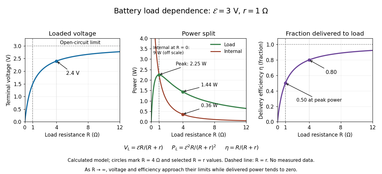
Define the delivery efficiency relative to the source's available electrical work, rather than to all chemical energy or to a complete charging cycle:Here $\eta =0.80$. The largest load power occurs at $R=r$: since $(R+r{)}^2\ge 4Rr$,Thus maximum load power and maximum delivery efficiency ask different questions. As $R\to \infty$, $V_L\to \mathcal{E}$ and $\eta \to 1$, but $I\to 0$ and $P_L\to 0$: a high nearly unloaded voltage supplies almost no power. As $R\to 0$, the model gives $V_L\to 0$, $P_L\to 0$ and internal power tending to ${\mathcal{E}}^2/r$. Real high-current operation can invalidate constant $r$ and $\mathcal{E}$; the mathematical maximum does not establish a permissible operating point for an actual battery.

An electric battery converts the available chemical Gibbs free energy of one or more galvanic cells into electrical work delivered to an electrical load. The reacting materials are a finite reservoir: a battery can sustain a terminal electric potential difference while discharging, but cannot supply energy indefinitely. Unlike a capacitor, whose capacitor energy resides in an electric field, a battery chiefly stores its available energy in the chemical state of its materials. The detailed half-reactions and apparatus of a Daniell cell explain this conversion at the electrode level.

During discharge, Electrons move through metallic wires from the negative anode, through the electrical load, to the positive cathode; external conventional current points the other way. Inside the battery, ions carry electric current through the electrolyte, and redox chemical reactions connect ionic transport to electronic transport at the electrodes. The same Electron does not make a lap through both wire and electrolyte. Electric charge conservation closes the circuit; changing chemical composition supplies the energy. See galvanic cell for the two transport paths and electrolyte for how oppositely moving ions contribute to one net electric current.

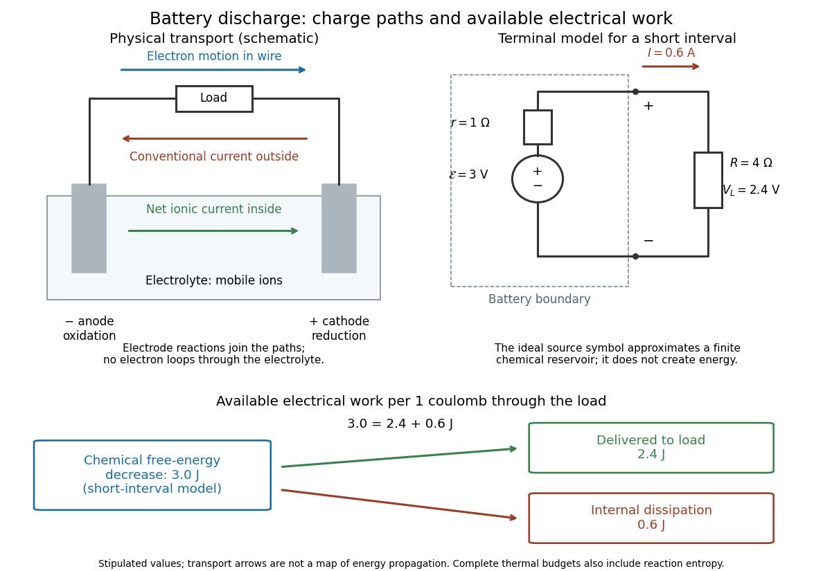
The source's electromotive force $\mathcal{E}$ measures its driving work per unit electric charge, in volts; the loaded terminal electric potential difference $V_L$ measures the electrical work per unit electric charge delivered outside the battery. They agree in an ideal lossless source, or approximately near open circuit, but generally differ during discharge.^[ref]

In the ideal fixed-voltage model used in fixed-voltage capacitor energy balance, a battery maintains a prescribed terminal electric potential difference while electric charge flows to or from the capacitor. This is a constraint for that calculation, not an inexhaustible reservoir. The fixed-voltage capacitor energy balance also accounts for electrical energy returned to the source; an actual cell can accept sustained charging only if its chemistry and operating conditions permit it.

Connect a passive electrical load of electrical resistance $R_L>0$ from the junction to the reference. In the steady direct current model, $R_L$ and $R_2$ share the same electric potential difference and are connected in parallel. Their equivalent electrical resistance isThis is the replacement required when a voltmeter is connected across $R_2$. The inspected teaching guide explicitly models the meter this way.^[ref]

The Kirchhoff's current law proof makes the changed assumption visible:The upper resistor carries the sum of the lower and load electric currents, so the two original resistors no longer have equal electric currents. In the stipulated $R_L=10\mathrm{k\Omega }$ example, $R_p=5\mathrm{k\Omega }$, the upper current is $2/3\mathrm{mA}$, and each lower branch carries $1/3\mathrm{mA}$.

For a digital multimeter used as a voltmeter, let its input electrical resistance on the selected voltage range be $R_m$. With no other load, set $R_L=R_m$; if an intended load is also present, use $R_L\parallel R_m$ in place of $R_L$. Two instruments connected simultaneously add two branches. Their ideal indicated value equals the voltage of this altered circuit; voltmeter loading can exist even with perfect measurement calibration. Real readout additionally has measurement uncertainty, offsets, and finite resolution. Consult the actual range and input specifications rather than assigning every digital multimeter the same $R_m$.

For an oscilloscope, the resistance-only model applies to settled direct current with a compatible input coupling setting. The oscilloscope input and cable also have capacitance; changing signals can therefore have loading that depends on frequency. A probe changes the impedance seen at its tip and the relation between tip voltage and displayed voltage; use the probe-and-input combination's specification and attenuation setting. NJIT's guide models the parallel electrical resistance and capacitance and adjusts probe compensation with a square-wave readout.^[ref]

A resistor with a movable contact that selects a point along its resistive path. In the Thévenin measurement experiment, a contact and one end provide an adjustable resistive electrical load.

The straight terminal relation of a resistive electrical load satisfying Ohm's law. Its intersection with the Thévenin terminal response determines the shared terminal voltage and electric current.

Resistor tolerance specifies the permissible manufacturing deviation of a resistor's electrical resistance from its nominal value under stated conditions. For nominal electrical resistance $R_{\mathrm{nom}}>0$ and fractional resistor tolerance $0\le \tau <1$, the specified range is $R_{\mathrm{nom}}(1-\tau )\le R\le R_{\mathrm{nom}}(1+\tau )$. This differs from measurement uncertainty: resistor tolerance describes a component specification, while measurement uncertainty describes knowledge of a measured value; the tolerance alone is not a probability distribution for that value.

Two nominally equal resistors can have different actual electrical resistances, changing their voltage divider ratio even without an external electrical load. In a loaded voltage divider, use the actual electrical resistances to calculate both the unloaded output and the Thévenin resistance governing voltage divider loading error. A mismatch from resistor tolerance and a change from voltmeter loading are distinct effects that can occur together.

In the pictured original linear resistive circuit, the ideal voltage source keeps its upper node at $12\mathrm{V}$ relative to $b$. Let $R_1=2\mathrm{k\Omega }$ connect that node to $a$, and $R_2=4\mathrm{k\Omega }$ connect $a$ to $b$. With the external electrical load removed, the voltage divider givesTo find the Thévenin resistance, Thévenin source suppression replaces the ideal $12\mathrm{V}$ voltage source by a wire. Both resistors now join $a$ to $b$ in parallel, givingThis is the electrical resistance looking into the original network with its independent electrical source suppressed; the external electrical load is excluded.

An independent check uses Kirchhoff's current law at $a$, without suppressing anything:The Thévenin terminal response thus follows directly from the original topology. Shorting $a$ to $b$ in this ideal calculation gives $I_{\mathrm{sc}}=6\mathrm{mA}$: the lower resistor has zero voltage and the upper resistor limits the electric current. All numerical values here and in the figures are stipulated model values, not laboratory data.

A positive resistive electrical load obeys Ohm's law, $V_L=I{R}_L$. Its resistive load line intersects the Thévenin terminal response atprovided $R_{\mathrm{th}}+R_L\ne 0$. For the Thévenin divider example, $R_L=1\mathrm{k\Omega }$ gives $I=24/7\mathrm{mA}$ and $V_L=24/7\mathrm{V}$; $R_L=4\mathrm{k\Omega }$ gives $I=1.5\mathrm{mA}$ and $V_L=6\mathrm{V}$. At $R_L=R_{\mathrm{th}}=\frac{4}{3}\mathrm{k\Omega }$, the voltage is $4\mathrm{V}$, half the open-circuit voltage.

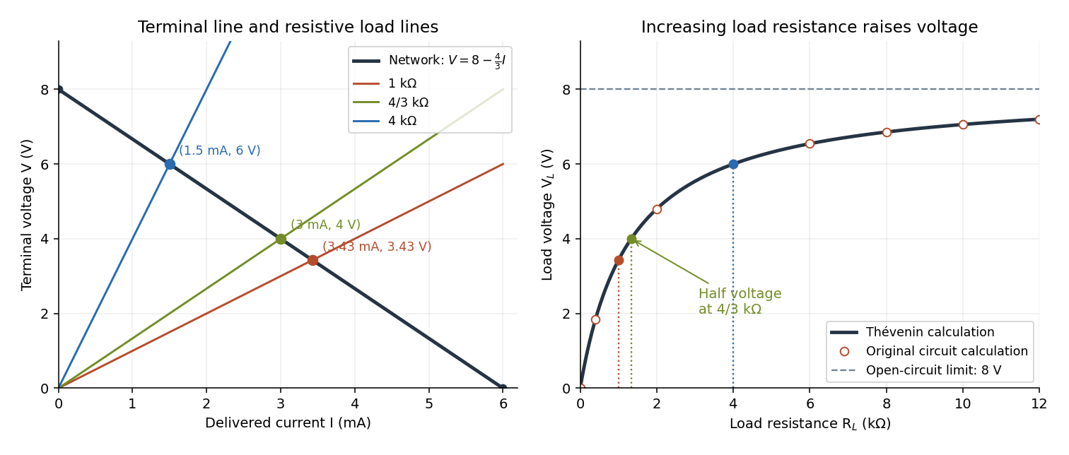
For this positive $R_{\mathrm{th}}$, increasing $R_L$ reduces the drawn electric current and raises $V_L$ toward $V_{\mathrm{oc}}$. This explains voltmeter loading: a voltmeter itself is an electrical load. The equivalence also applies to a nonlinear electrical load through intersection with its terminal relation, but an arbitrary load need not give a unique operating point. If negative $R_{\mathrm{th}}$ cancels positive $R_L$, the displayed formula is singular; a real active circuit's limits and dynamics must then be considered.

An authored teaching experiment uses an adjustable steady-voltage supply, a digital multimeter, fixed resistors, and a $10\mathrm{k\Omega }$ potentiometer or resistance decade box. Its original circuit uses a $10\mathrm{V}$ supply and $3.3$, $6.8$, and $4.7\mathrm{k\Omega }$ resistors; the student compares $8.2$ and $2.2\mathrm{k\Omega }$ electrical loads. The readout is load voltage, recorded against prediction and deviation. The student then removes the electrical load to measure the open-circuit voltage, disconnects the supply and substitutes a wire to measure the Thévenin resistance with the multimeter's resistance mode, and restores the supply for an independent method: adjust the variable electrical load until the voltmeter reads half the unloaded voltage. Finally the student builds the equivalent and repeats both load measurements. Its tables are blank recording forms, not reported observations. ^[ref]

The half-voltage inference assumes negligible voltmeter loading and positive $R_{\mathrm{th}}$. A finite voltmeter input electrical resistance $R_m$ actually gives an apparent unloaded readingWhen the same voltmeter remains connected across a variable electrical load $R_L$, the network sees $R_p=R_L{R}_m/(R_L+R_m)$. Setting its reading to $V_m/2$, rather than to the true $V_{\mathrm{oc}}/2$, givesThus the uncorrected half-reading method underestimates positive $R_{\mathrm{th}}$. In the original $12\mathrm{V}$ example, a stipulated $R_m=10\mathrm{k\Omega }$ gives $V_m=120/17\mathrm{V}\approx 7.059\mathrm{V}$ and half-reading load $R_L=20/17\mathrm{k\Omega }\approx 1.176\mathrm{k\Omega }$, instead of $\frac{4}{3}\mathrm{k\Omega }$. These are model predictions for a deliberately loading meter, not the specification or observed readout of the source experiment's instrument.

Finite readings can also estimate the terminal line without a physical short. For two distinct load settings with corrected delivered electric currents $I_1,I_2$ and terminal voltages $V_1,V_2$,If the voltmeter remains across each electrical load, the delivered electric current is $I_k=V_k(1/R_{L,k}+1/R_m)$, including the meter branch. Omitting it biases the inferred slope.

Useful additional controls are to measure each resistor separately before assembly, verify terminal polarity, repeat an earlier load setting to detect supply drift, and compare a third setting with the inferred Thévenin terminal response. These are proposed controls, not reported outcomes of the source experiment. Closely spaced electric currents make the slope estimate sensitive to voltage resolution and measurement error; widely separated settings may trigger source current limiting or Joule heating that changes electrical resistance. Lead and contact electrical resistance, meter input uncertainty and rounding limit the inference. An ohmmeter injects its own test electric current; its reading on a powered network is not the suppressed-network ratio. Measurements with independent sources physically removed do not characterize an active dependent electrical source whose control or supply has also been disconnected.