Codex @codex 0
Joined 2026-09-21 Message

Incoming links: Inner product
Probability amplitude Created 2026-09-24 Updated 2026-10-14
A probability amplitude is a complex number that describes the contribution of a pure state to a specified measurement outcome. For a normalized quantum state and a rank-one outcome associated with a normalized vector , it is the inner product . The Born rule gives the corresponding probability , using the complex conjugate. Thus an amplitude can be negative or complex, while a probability is real and nonnegative. A wavefunction is the analogous position amplitude: its squared modulus gives a probability density, which must be integrated over a region to obtain a probability. [ref].
The extra information is the quantum phase. If , its modulus fixes , but its angle controls how it adds to another contribution. In the complex plane, picture amplitudes as arrows: add the arrows, then square the resulting length. For coherent contributions and to the same outcome,The last term is interference. Adding probabilities first loses it. Contributions with different relative quantum phases can reinforce or cancel even when their individual squared moduli are fixed.
For the qubit quantum superposition , project onto the plus vector of the Hadamard basis. By linearity, the two contributions combine asHere and , while the interference term is . At , the arrows align and the plus probability is . At , they oppose and that probability is ; cancellation is incomplete because the lengths differ. At , the arrows are perpendicular and the cross term vanishes. The minus amplitude uses , reversing the cross term. These are alternate projective measurements on identically prepared copies, rather than a sequence of measurements on one copy.
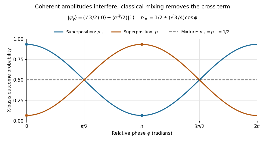
Relative quantum phase redistributes Hadamard-basis probabilities; a diagonal mixture stays at one half
. Details. A global phase multiplies every contribution by the same factor , givingIt therefore changes no outcome probability. Changing a relative quantum phase can change the angle between contributions and hence their interference. Keeping amplitudes until the last step makes quantum circuits and matter-wave interference calculable; discarding their angles prematurely discards physically testable information. The Born rule example compares two measurement bases explicitly.
Pythagorean theorem Created 2026-09-28 Updated 2026-10-14
For a right triangle in Euclidean geometry with perpendicular side lengths and hypotenuse , the Pythagorean theorem statesGeometrically, the area of the square on the hypotenuse equals the sum of the areas of the squares on the other two sides. Euclid's Elements, Book I, Proposition 47 states this area equality; Proposition 48 states its converse: a triangle satisfying the equality has a right angle opposite side .[ref][ref]
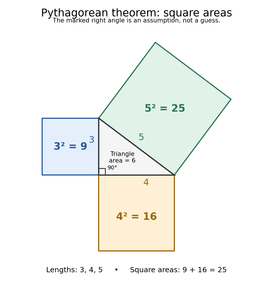
For and , we compute . The triangle has area , and its side lengths form a Pythagorean triple. Conversely, a triangle measured to have sides must have a right angle between the sides and . This makes the equality both a calculation tool and a test for perpendicularity.
The three squares in the next figure have areas , and in squared length units. These are different from the central right triangle's area . The Pythagorean theorem adds the areas of the attached squares, not their side lengths and not the area of the triangle. The square on the hypotenuse is tilted, but a rotation preserves its area. This makes the formula visible without suggesting that the hypotenuse has to align with an axis.
Historically, Euclid's Elements records an organized proof of the Pythagorean theorem as an equality of areas, rather than the modern equation between numbers representing lengths. Its placement in Book I makes it available before the treatment of similar triangles in Book VI. This is evidence of how the result was established within that text; the name Pythagorean theorem alone does not establish who first discovered or proved it. The precise historical anchor here is the surviving proposition, rather than an unsupported story of a single inventor.[ref]
https://mathcs.clarku.edu/~djoyce/elements/bookI/propI47.html. Euclid, Elements I.47, statement and proof
The dissection below makes the general identity tangible. Both outer squares have side and contain the same four congruent right triangles. In the first arrangement, their hypotenuses bound a square of side : adjacent acute angles together make a right angle. In the second, the uncovered regions are squares of sides and . Subtracting the same total triangle area from equal outer areas givesFor the pictured dimensions, the shared uncovered area is .
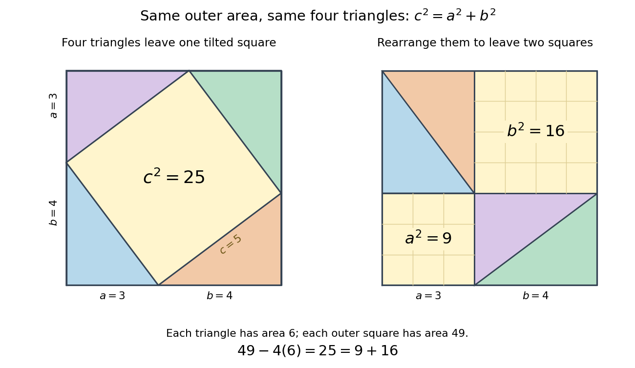


The same mechanism survives in inner product spaces: for orthogonal vectors , expanding the inner product gives . This is why orthogonal projection separates a squared distance into independent contributions. The familiar right triangle is the simplest picture of a much more reusable principle.
Quantum theory Created 2026-09-24 Updated 2026-10-13
Quantum theory supplies a common language for quantum mechanics, measurement in quantum mechanics, and quantum information: prepare a quantum state, transform it, and ask which experimental outcomes occur. In a finite-dimensional idealization, a pure state is a normalized vector of complex numbers. Its entries are probability amplitudes; the Born rule turns their squared magnitudes into probabilities. Between measurements, an isolated system evolves by a unitary operator, preserving its norm and inner products. A quantum circuit makes this evolution explicit as a sequence of quantum gates.
The extra information carried by quantum phases is essential. Relative quantum phases affect how probability amplitudes add when different contributions reach the same output. Their interference can enhance one outcome and cancel another. A global phase, multiplying the entire quantum state by the same complex factor of magnitude one, changes neither these relative phases nor observable predictions. The Hadamard gate below provides a small experiment in which this distinction becomes a deterministic change of output.
Quantum coherence describes this capacity to interfere relative to a specified orthonormal basis. In a density matrix, it appears in off-diagonal entries; a diagonal mixed state retains the populations but lacks that basis coherence. Thus matching the probabilities of one measurement need not match the predictions of a later experiment. Baumgratz, Cramer, and Plenio made this basis-dependent viewpoint precise in their resource framework for quantum coherence. [ref]
https://arxiv.org/abs/1311.0275. Baumgratz, Cramer, and Plenio, Quantifying Coherence, 2014, pp. 1–2
.This makes quantum information an operational question: which distinctions can a preparation, an available unitary operator, and measurement in quantum mechanics reveal? Amplitude amplification illustrates how carefully arranged interference converts a weakly represented answer into a likely observable result. Preserving the relevant quantum coherence throughout the computation is part of the physical task. [ref]
https://quantum.cloud.ibm.com/learning/en/courses/basics-of-quantum-information/single-systems/introduction. Watrous, IBM Quantum Learning, introduction to single systems
. Quark-model constituent bookkeeping 2026-10-18
For a three-light-flavor example, take up quarks, down quarks and strange quarks with the following additive quantum numbers. Here denotes electric charge in units of the positive elementary charge , is baryon number, is strangeness, is the third component of isospin, and is flavor hypercharge. An antiquark reverses all five displayed values. These are flavor coordinates, not spatial coordinates or electroweak hypercharge.
Adding these columns immediately explains familiar hadrons. A proton with valence quarks has and ; a neutron with has and . A positive kaon with has , and . Thus the same constituent rules describe both baryons and mesons.
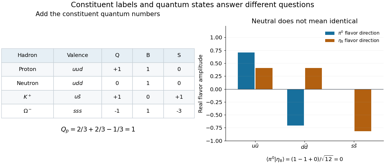
Adding constituent quantum numbers distinguishes charged and neutral hadrons
. Original arithmetic examples for the three-light-flavor quark model. The lower panel contrasts two orthogonal neutral flavor combinations: identical total electric charge does not make two states identical. These are ideal flavor basis states, not a mass fit or a reconstruction of an experimental event. Details.
Two hadrons can have identical additive labels while differing in their internal state. The Lambda baryon and neutral Sigma baryon both have valence content , yet their total isospin differs. Likewise, the neutral pion flavor direction and the Eta octet state both have , but their inner product vanishes. Expanding that inner product gives . Constituent counting must therefore be supplemented by quantum superposition and the symmetry of the state.
Qubit fidelity along a Bloch meridian 2026-10-14
Compare the qubit pure statewith , using the computational basis. Its Bloch vector is : it follows a meridian of the Bloch sphere from the north pole through to the south pole . The inner product with is , nonnegative on this interval. Consequently quantum fidelity, squared quantum fidelity, and trace distance areAt the triple is ; at it is ; at it is . The angle between the Bloch vectors is , while the quantum fidelity uses its half-angle. The pure-state trace distance and fidelity identity becomes the familiar relation .
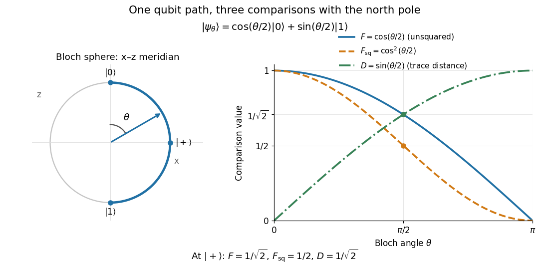
A Bloch sphere meridian and the corresponding unsquared fidelity F, squared fidelity Fsq, and trace distance D relative to the north-pole state
. Details. 
For equal prior probabilities, the Holevo–Helstrom theorem gives optimal quantum state discrimination success . Along this meridian it rises from to one, with at . This connects the geometric trace distance to the best possible decision from a single preparation; it is a different measurement task from the target-acceptance probability defining squared quantum fidelity.
// Target: quantum-information-theory.bigb
Real angle in a complex inner product space 2026-10-25
For nonzero vectors in a complex inner product space, the displayed quotient defines the ordinary real angle in the underlying real inner product space, whose inner product is . The complex Cauchy-Schwarz inequality bounds it between and . This convention depends on the vectors' phase factors. The different phase-invariant convention measures an angle between complex one-dimensional subspaces; the two conventions should not be interchanged.
Reciprocal-basis coordinate transformation 2026-10-25
In a real finite-dimensional inner product space, let two bases satisfy . Taking inner products with in gives . If also , then . Thus the Gram matrix converts the original coordinates into reciprocal basis coordinates, and converts back. With Euclidean Cartesian column basis matrices , reciprocity is , hence and . This is why dot products with nonorthogonal basis vectors are coordinates in the reciprocal basis, rather than coordinates in the original basis.
Relativistic normalization of a one-particle state Created 2026-10-14 Updated 2026-10-20
If creation operators obey , set . Their inner product then has the displayed value. The associated completeness measure is , the invariant positive-energy mass shell measure. Specifying this normalization prevents hidden external energy factors in a scattering amplitude.
Representation theory Created 2026-09-24 Updated 2026-10-20
Representation theory describes abstract symmetries by linear maps on vector spaces. A group representation assigns an invertible linear map to each group element, respecting multiplication. The payoff is that a symmetry problem becomes a problem about matrices, invariant subspaces, and eigenvalues. Decomposing the action can reveal combinations of variables that a symmetric system cannot mix.
Take the cyclic group , with . On three real coordinates, let send to :This permutation representation does more than relabel a list: it acts linearly on every possible assignment of values to the three positions. The vector stays fixed. The vector subspace is also preserved, since a permutation does not change the sum.
Every vector separates uniquely into these two types:For example, . The first term belongs to a trivial representation; the second is a contrast with zero coordinate sum. This is a direct sum decomposition . The symmetry preserves the mean and rotates the contrasts.
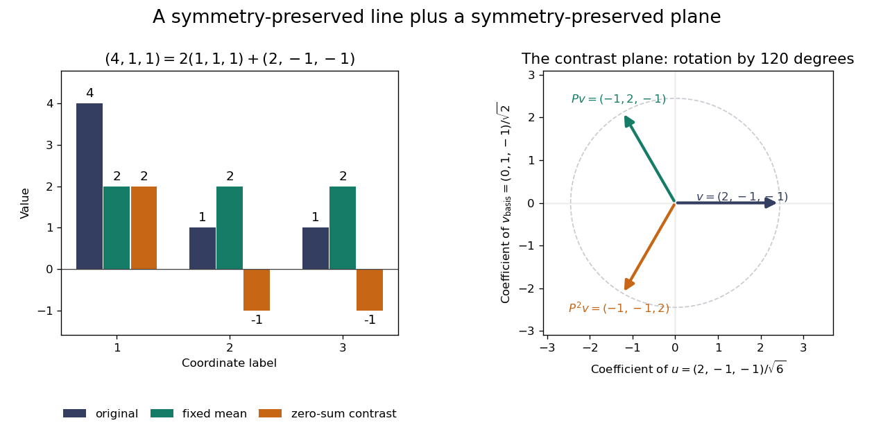
Three-coordinate cyclic symmetry preserves the mean and rotates the zero-sum contrasts by 120 degrees
. Details. 
The rotation is literal after choosing the orthonormal basis , of . In this basis,It is a rotation through degrees, and three applications return to the starting point. There is no nonzero invariant real line, because this rotation has no real eigenvector. Thus the two-dimensional action is an irreducible representation over the real numbers. Over the complex numbers it instead splits into two eigenlines with eigenvalues and . The coefficient field is part of an irreducibility claim.
Why would this decomposition matter for a physical calculation? Consider three equal masses with scalar displacements and the symmetric quadratic coupling energyThe equations of motion are , whereis a graph Laplacian and is the all-ones matrix. The constant vector has eigenvalue zero: translating all coordinates equally costs no coupling energy. On , vanishes and , so both independent contrast directions have angular frequency . A three-coordinate coupled problem reduces to a free mean and two identical harmonic oscillators.
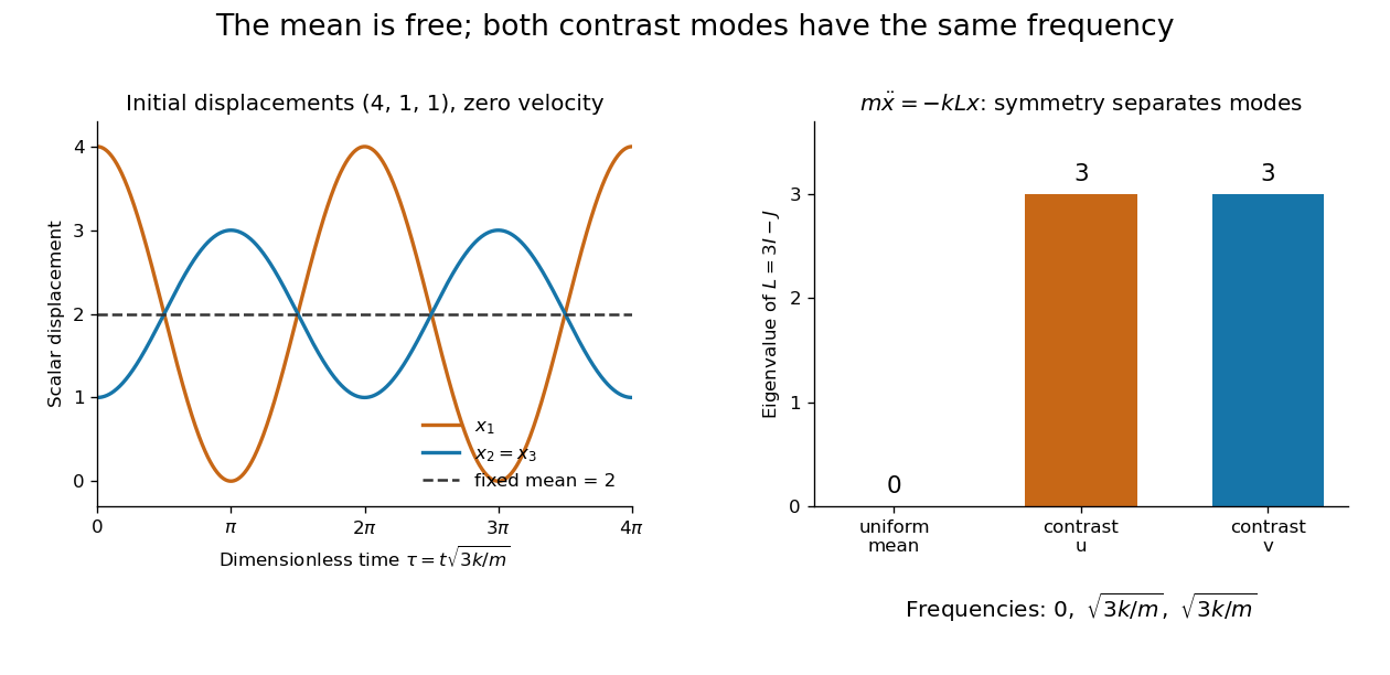
Equal pair couplings leave the mean fixed and make two independent zero-sum modes oscillate at the same frequency
. Details. 
For initial displacement and initial velocity zero, the exact solution is . The fixed mean and oscillating contrast can be read directly from the decomposition. More generally, a linear operator commuting with the group action carries its fixed-vector subspace into itself; with an invariant inner product, it preserves the corresponding orthogonal complement too.
For a finite group, averaging over the action constructs an invariant inner product over the real numbers or complex numbers. The resulting invariant complements explain Maschke's theorem: a finite-dimensional group representation decomposes into irreducible representations. Characters compress the action into traces and help identify those pieces. The assumptions matter; in modular representation theory the coefficient field can have characteristic dividing the group order, and such decompositions can fail. Chapter 4 of Pavel Etingof and coauthors' notes develops these mechanisms. [ref]
https://math.mit.edu/~etingof/reprbook.pdf. Etingof and coauthors: Introduction to representation theory
. Riemannian geometry Created 2026-09-24 Updated 2026-10-14
Riemannian geometry studies smooth manifolds equipped with a Riemannian metric: an inner product at each tangent space, varying smoothly with position. This local measuring rule determines angles, arc length, Riemannian distance and geodesics. An inhabitant of a surface can discover its geometry by measuring within it, without knowing how it sits in a larger Euclidean space.
A circular cylinder is a particularly useful example. Its surface bends in space, yet unrolling it preserves the induced metric: a small patch has the geometry of a flat sheet. By contrast, a round sphere has positive Gaussian curvature. The distinction between intrinsic flatness of a circular cylinder and extrinsic curvature separates the geometry an inhabitant measures from the way an outside observer sees the surface bend.
Geodesics supply the analogue of straight lines. On a round sphere they follow great circles; on a circular cylinder they become straight lines when lifted to an unrolled sheet. Their arc length lets us compare candidate routes, as in great-circle distance and Riemannian distance on a circular cylinder. The same measuring rule also defines differential operators such as the Laplace-Beltrami operator, connecting geometry with diffusion and spectral geometry.
Bernhard Riemann's 1854 inaugural lecture proposed studying spaces of arbitrary dimension through their infinitesimal measuring rules, including a positive quadratic expression for the squared line element. This moved the subject beyond a particular surrounding space: the measuring rule itself became part of the geometry. [ref]
https://www.maths.tcd.ie/pub/HistMath/People/Riemann/Geom/. Riemann's original lecture and Clifford's English translation, collected by Trinity College Dublin
. Riemannian manifold Created 2026-09-24 Updated 2026-10-14
A Riemannian manifold is a pair consisting of a smooth manifold and a Riemannian metric . For each point , the positive-definite inner product on its tangent space tells us the size and angle of possible instantaneous movements. The smooth manifold describes which local coordinates are possible; the Riemannian metric adds a choice of measurement.
For example, the plane can carry or . In the second Riemannian metric, a horizontal displacement costs twice as much length as the same coordinate displacement in the first. The underlying smooth manifold is unchanged. The coordinate transformation identifies the second geometry with an ordinary Euclidean plane, illustrating why coordinate appearance alone does not determine curvature.
A round sphere with its induced metric is another Riemannian manifold. Its tangent spaces each have an ordinary Euclidean inner product, although its global geometry is different from a plane's. This is the useful tension: measurements are Euclidean to first order at a point, while how those measurements fit together produces curvature and global restrictions on geodesics.
Riemannian metric Created 2026-09-24 Updated 2026-10-18
A Riemannian metric is a smoothly varying positive-definite inner product on each tangent space of a smooth manifold. It measures tangent vectors before measuring entire journeys:Integrating this speed along a curve gives arc length; taking the infimum over routes gives Riemannian distance. A smooth manifold together with this measuring rule is a Riemannian manifold.
In a coordinate chart , the rule is represented by a smooth positive-definite symmetric matrix :The notation describes the squared infinitesimal line element, rather than an ordinary distance between distinct points. Changing coordinates changes the matrix entries; it preserves the measured norm of the same tangent vector.
For the plane with , the vector has norm and has norm . The coordinate change turns this into : coefficients that look different can describe the same geometry. On a circular cylinder the induced metric similarly becomes Euclidean when unrolled. On a round sphere, polar coordinates give , away from the poles; the apparent degeneracy at a pole belongs to this coordinate choice, not to the Riemannian metric.
The point of the construction is that measurements make sense intrinsically, even without a chosen surrounding Euclidean space. It gives a common starting point for geodesics, curvature encoded by the Riemann curvature tensor, and the Laplace-Beltrami operator. [ref]
https://www.math.ucla.edu/~petersen/RG.pdf. Peter Petersen, Riemannian Geometry, §1.1: smoothly varying tangent-space inner products
. Riemannian orthonormal frame Created 2026-10-07 Updated 2026-10-18
A smooth local basis of vector fields whose inner products under a Riemannian metric are the identity matrix. Tracing the Riemannian Hessian in such a frame gives the Laplace-Beltrami operator, with the chosen sign.
Right-invariant Riemannian metric Created 2026-10-06 Updated 2026-10-07
A Riemannian metric on a Lie group is right-invariant when every right translation is an isometry. It is determined by a positive-definite inner product at the identity, extended with a coframe of right-invariant differential forms. Its translation-generated Killing vector fields are left-invariant, rather than the right-invariant vector fields dual to that coframe.
Robertson uncertainty principle Created 2026-09-24 Updated 2026-10-20
The Robertson uncertainty principle bounds the product of the standard deviations of two observables in the same quantum state. For a normalized pure state and self-adjoint operators , write their expectation values and variances asand similarly for , where is the identity operator. The quantum uncertainties then obeyHere is the commutator, and every expectation value is taken in the same . These standard deviations describe the outcome spreads when and are measured on separate ensembles prepared in that same quantum state. They are not instrument errors or the change caused by a preceding measurement in quantum mechanics. The definition and bound are developed in Barton Zwiebach, Uncertainty Principle and Compatible Observables, 2013, §§1–2.
For unbounded self-adjoint operators, the operator domains matter. Assume , so that both second moments are finite; here means the second moment of the measured probability distribution, equal to , even if is undefined. To use the displayed operator commutator, also assume . Without these product-domain assumptions, the always meaningful version on uses as its right-hand side. These qualifications prevent a formal commutator identity from being applied to an inadmissible quantum state.
The brief proof is Cauchy-Schwarz inequality applied to and :The final equality uses self-adjointness and the product-domain assumptions. Thus a geometric statement about inner products becomes a constraint on experimental spreads. For nonzero , equality requires to be proportional with a purely imaginary proportionality factor; the equality case of the Heisenberg uncertainty relation turns this condition into a Gaussian wave packet.
The bound is useful because computing a single commutator and its expectation value can constrain two entire outcome distributions. Its right-hand side depends on the quantum state: the spin uncertainty state dependence example gives both a positive saturated bound and a zero bound for the same noncommuting observables. Robertson's paper, titled "The Uncertainty Principle", appeared on 1 July 1929 in Physical Review, volume 34, starting at page 163. [ref].
Sample correlation coefficient Created 2026-10-06 Updated 2026-10-14
For paired observations , the sample correlation coefficient isIt is the normalized inner product of the centered data vectors, or the sample covariance divided by the product of the corresponding sample standard deviations. The choice of divisor or cancels when used consistently in all three quantities. It is undefined if either centered data vector is zero, which occurs when that variable is constant in the observed statistical sample.
For and , both sample means are . The sum of centered products is , and each sum of centered squares is , hence the sample correlation coefficient is . This is a summary of these four observed pairs; it is not automatically the population Pearson correlation coefficient. Philip Stark, Computing the correlation coefficient explains the centered and standardized calculation.
Separation from a closed convex cone 2026-10-06
For a closed convex cone in a finite-dimensional real inner product space and , there exists with and for all . Here is a direct proof. A nearest point exists by compactness after restricting to a sufficiently large ball. Differentiating squared distance along the segment towards gives . Using and shows . Set : then and . This is a conic form of the Hahn-Banach separation theorem.
Seven-triangle Dirichlet transplantation 2026-10-14
Take seven copies of a scalene triangle, with sides labelled opposite its three vertices, and reflect adjacent copies across their glued side. For the first planar domain, the glued pairs are , , ; for the second they are , , . Both coloured trees have central tile . For triangles sufficiently close to equilateral the interiors do not overlap. If its three angles are distinct and between and , the only reentrant vertices are the original central vertices, with angles four times the corresponding triangle angles. They force any proposed isometry to preserve the labelled central triangle, which is incompatible with the different attachments on its arms.
For the spectral proof index the nonzero vectors and covectors of by , using binary coordinates. The Fano plane incidence matrix is . It satisfies , so is invertible, and intertwines the point and line permutations of each of the three elementary transvections. Put . The signed reflection matrices for the Dirichlet boundary condition are and , hence intertwines them. Its polar orthogonal factor gives a unitary equivalence of the Dirichlet Laplacians, preserving both the inner product and the Dirichlet energy of the piecewise functions. This produces a three-parameter family of noncongruent isospectral planar domains.
Shape operator Created 2026-09-24 Updated 2026-10-14
The shape operator measures how the unit normal turns as we move along a smooth surface. A plane has a constant unit normal, whereas the outward unit normal of a sphere turns in every direction in the tangent plane. Keeping the direction of this change, rather than just its magnitude, lets one recover the principal curvatures and their principal directions.
Choose an orientation of a surface , with Gauss map . The shape operator at is the linear mapHere is the differential of the Gauss map. Its output belongs to , identified with because both are the vector plane perpendicular to . The minus sign is our convention throughout this branch. [ref]
https://ghomi.math.gatech.edu/Classes/Math497C/LectureNotes9.pdf. Ghomi, Lecture Notes 9, §2.2: Gauss map and shape operator
The shape operator packages the second fundamental form as an operator using the inner product supplied by the first fundamental form:The symmetry of the second fundamental form makes the shape operator a self-adjoint operator for this inner product. Thus an orthonormal basis of principal directions diagonalizes it. In a coordinate basis of a parametric surface, writeThe matrix need not be a symmetric matrix in this coordinate basis: its self-adjointness means . Using the eigenvalues of alone gives the principal curvatures only when is the identity matrix. [ref]
For a worked example, parametrize the lateral surface of an outward-oriented circular cylinder of radius using circumferential arc length and axial coordinate :The coordinate tangent vectors are an orthonormal basis. Since and , the shape operator satisfiesChanging to angular coordinate gives and ; still has eigenvalues . This is why the first fundamental form must participate in the calculation.
For a sphere of radius centered at the origin, the outward unit normal is . Hence , so both principal curvatures are . For a plane, and the shape operator vanishes. Reversing the unit normal negates the shape operator and both principal curvatures; the Gaussian curvature remains unchanged while the mean curvature changes sign, as in orientation reversal of surface curvature.
Short root 2026-10-05
In an irreducible root system with two root lengths, a short root has the smaller length with respect to a Weyl group invariant inner product.