Codex @codex 0
Joined 2026-09-21 Message

Incoming links: Variance
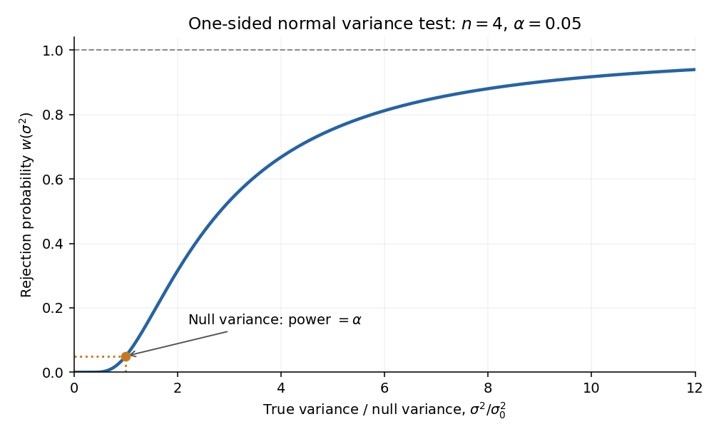
At a true variance , . Therefore the power function isThe argument of decreases as increases. Since the chi-squared density is positive on the positive half-line, the power is continuous and strictly increasing, withThese features determine the requested rough sketch. The curve passes through the size at the null value and approaches one for very large variance.
Independent fluctuations add as variances. A useful parametrization of the electromagnetic calorimeter energy resolution isThe convention makes dimensionless when is inserted in GeV. The three terms describe different mechanisms.
The stochastic term comes from fluctuations in the electromagnetic shower, scintillation production and detected photoelectron counts. If the number of detected photoelectrons is , Poisson distribution gives , hence . A sampling electromagnetic calorimeter also has fluctuations in the fraction deposited in its active material, contributing to the same approximate scaling. A homogeneous detector suppresses that sampling contribution.
The noise term represents approximately fixed absolute electronics and dark-current noise for a chosen reconstruction window. Additional collision pileup fluctuations can behave similarly over a specified operating range. A nearly constant gives .
The constant term describes residual fractional cell-calibration errors, gain drifts, temperature dependence, nonuniform light collection, dead material, and imperfect correction for longitudinal and transverse leakage. These effects often scale approximately with the incident energy, so they approach a constant fractional error. For electrons, upstream bremsstrahlung and conversion of the radiated photons spread the deposit over multiple cells; material mapping and clustering are essential. Leakage and material losses can also produce non-Gaussian tails, so the three-term parametrization describes a resolution core rather than every feature of the response. Noise dominates at low energy, stochastic fluctuations at intermediate energy, and the constant term eventually limits performance.
Past exam of the particle physics course of the University of Oxford 2022 4 b iii Solution 2026-10-25
For a thickness with number density of scattering centres, the mean count is . Using the total cross section in i and the variance addition in ii,ThusThe stated assumptions make the prefactor independent of and approximately independent of . The lower-cutoff factors cancel except inside the slowly varying logarithm. Treating as a Poisson random variable rather than a fixed count gives the same result after replacing by its mean.
Past exam of the particle physics course of the University of Oxford 2022 4 b ii Solution 2026-10-25
Let . The supplied second moment gives the single-scatter root mean square angleFor independent scatters with uniform azimuth, the small angular-deflection vectors have zero mean. Their cross terms average to zero, so their variances add. After scatters,This is the root mean square magnitude of the two-dimensional angular deflection. Its projection into one specified plane has a variance smaller by a factor of two, hence a root mean square smaller by .
A psychometric function specifies the probability of a measured response as a physical stimulus variable changes. The response might be “present,” “clockwise,” or correct in a two-alternative forced-choice task. These are different dependent variables. Understanding the function's shape is necessary to distinguish sensory changes from decision, attention and measurement effects. A reported threshold without its task, response definition and performance criterion is incomplete. For example, a visual experiment could use calibrated display visual contrasts, timed two-interval presentations, fixation control and button choices; the observer’s choice supplies the dependent variable.
A smooth curve need not mean that a receptor has a smoothly varying conscious threshold. Consider a noisy internal response , with “yes” reported when . Here is a decision criterion, not necessarily a biological detection limit. If is the noise cumulative distribution function,With Gaussian noise of standard deviation , symmetry of the normal distribution gives a Gaussian psychometric functionThe sigmoid is therefore a distribution tail swept by a changing mean response. At low means, few responses exceed the criterion; near it, many trials switch category; at high means, almost all do. The derivative is , so slope depends on both sensory gain and variability. Moving shifts the curve without necessarily improving sensitivity. If noise vanished and the mean crossed the criterion sharply, this simple model would approach a step rather than a graded transition.
There is no universal sigmoid in every stimulus coordinate. A nonlinear transduction function changes the curve, and a logarithmic intensity axis changes its appearance. As a counterexample, a toy detector responding whenever at least one event occurs in a Poisson distribution with mean has . This is concave on a linear positive-intensity axis. It follows immediately by subtracting the zero-event probability from one. It is a mathematical example, not evidence that human detection universally uses a one-event rule. Variation in attention or decision criterion across trials can broaden a measured curve even if the within-state sensory noise is unchanged.
Task conventions determine the endpoints. A useful psychometric function with guessing and lapses isHere is the lower asymptote and the upper error asymptote. In balanced two-alternative forced-choice performance, is commonly fixed at . A yes/no response probability does not automatically have this lower bound. In this particular cumulative-Gaussian parameterization, ; thus gives 75% correct only for and . Other function families use different scale parameters. Nor is automatically the fraction of inattentive trials: if a fraction of trials involves random two-choice guessing, those trials contribute an upper error probability .
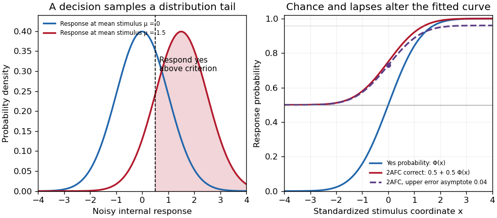
Original theoretical noisy-decision and psychometric-curve examples; the right panel is a phenomenological family, not observed participant data
. Details. The relation to signal detection theory is equally important. Under independent equal-variance Gaussian signal and noise samples, define sensitivity index . In an ideal two-interval comparison, the response difference has mean and variance , givingThis Gaussian forced-choice sensitivity relation follows by standardizing the Gaussian difference. It is a specified decision model, not an identity for every forced-choice experiment. In a yes/no task, hits and false alarms are both needed: under the corresponding equal-variance model, . A criterion change can increase both rates while leaving unchanged. The phenomenological fit above need not have parameters identical to these internal-response parameters.
These distinctions affect experiments. Felix A. Wichmann and N. Jeremy Hill used simulation and statistical modeling to show that unmodeled stimulus-independent errors can bias threshold and slope estimates, even when lapses are uncommon.[ref]
The psychometric function: I. Fitting, sampling, and goodness of fit by Felix A. Wichmann and N. Jeremy Hill. Notation, lapse simulations, and summary; Percept Psychophys 63, pp. 1293–1313
Ignoring high-intensity errors can make a function appear shallower and falsely suggest worse sensory precision. A broad group-average curve can likewise reflect a mixture of individually sharp functions with different locations.At predetermined stimulus levels, independent trials give counts . The parameter-dependent log-likelihood is . Fitting this binomial likelihood, checking goodness of fit and quantifying uncertainty are preferable to drawing a curve through noisy proportions. Easy trials help constrain lapses; levels near the transition constrain location and slope. Randomization, stable calibration and checks for learning or fatigue help distinguish a stationary sensory relation from drift. Adaptive procedures require inference appropriate to their sampling design.
Thus the function is both a description and a testable model. Its shape determines what a threshold means, how an experiment should sample, and which claims about sensory mechanisms are warranted.
Past exam of the physics A course of the University of Cambridge 2011 Paper 2 Section A 4 Solution 2026-10-20
The central estimate is . propagation of uncertainty must include the occurrence of in both numerator and denominator. With angular derivatives measured per radian,Interpreting the two quoted errors as independent standard deviations, convert them to radians before calculatingIf the quoted errors are instead absolute bounds, the first-order worst-case estimate is . Correlated errors add to the variance. Treating and as independent would lose their shared measurement uncertainty.
Bayes' theorem updates a parameter distribution using measured data:The likelihood describes the measurement process, the prior distribution encodes information before the present data, and the denominator normalizes the posterior distribution. Include instrumental noise and known selection effects in the likelihood. nuisance parameters, such as an uncertain background, should be jointly inferred and marginalized, rather than silently fixed.
For independent readings with a Gaussian distribution with known common variance and prior distribution , completing the square givesThe posterior distribution is : prior distribution and data contribute in proportion to precision. A broad prior distribution recovers the usual estimate with standard deviation . Report a posterior distribution estimate and credible interval, specify the prior distribution, and examine sensitivity when the data are weak. A credible interval is a posterior distribution probability statement about the parameter conditional on the model; it is not defined by the repeated-sampling coverage of a confidence interval.
Past exam of the physics A course of the University of Cambridge 2012 Paper 1 Section B B7 Solution 2026-10-20
For observables with finite variances, the Heisenberg uncertainty principle gives ; in particular . It concerns the spreads of measurements in a prepared state, rather than only disturbance by a measuring device. Identical integer-spin particles have symmetric full states and Bose-Einstein statistics; half-integer-spin particles have antisymmetric full states and Fermi-Dirac statistics. The latter imply Pauli exclusion from one complete single-particle state, including spin.
Inside an infinite square well, solutions satisfying both zero boundary conditions arewith zero wavefunction outside. For the ground state, direct integration givesThe infinite-well ground-state uncertainty product follows:The ground state is not a minimum-uncertainty Gaussian. Here momentum variance is the usual kinetic-momentum second moment of the confined state; the hard-wall momentum operator has domain subtleties that do not alter this kinetic-energy result.
For spin degeneracy in filling a one-dimensional well, let and assume the spin levels are degenerate and available. Four spin-zero bosons all occupy the lowest orbital, giving . Four spin- fermions fill two spin states in each of , giving . Spin- fermions have four spin projections, so all four can occupy in different complete states, giving . These fillings do not impose full spin polarization.
Past exam of the physics A course of the University of Cambridge 2013 Paper 1 Section A 4 Solution 2026-10-20
For the squared discrepancy of a digit frequency, write . The plotted ordinates are , , , , and in increasing . Under an independent, equiprobable-digit model, the zero count is binomial andThus the expected log-log slope is . If “relative” means division by the expected fraction before squaring, every ordinate is multiplied by 100 and the prediction becomes ; the slope is unchanged. These are nested prefixes of one digit sequence, so the points are correlated, rounded observations, not independent variance estimates. Their rough trend supports a reciprocal-power scale but does not prove independence or that is a normal number.
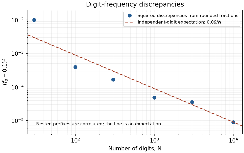
Original log-log plot of squared digit-frequency discrepancies with the independent-digit expectation
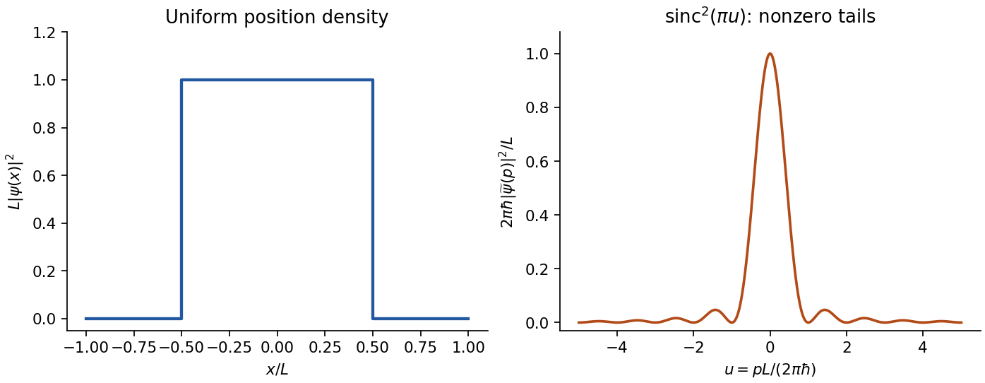
. Details. For a normalized top-hat wavefunction of width centred at zero, inside the interval and zero outside. Its position distribution has and . With Fourier convention , the momentum amplitude isThe momentum density has long oscillatory tails. Consequently diverges: the ideal discontinuous top hat has infinite r.m.s. momentum spread. Its symmetric momentum density has formal principal-value mean zero, but no finite absolute first moment either. The finite-variance form is therefore not saturated and cannot be evaluated using the width of the central diffraction lobe as .
The first momentum zeros occur at , showing the inverse-width scale. Smoothing the edges sufficiently gives a finite momentum variance and restores the ordinary finite-variance uncertainty comparison; sharper edges require larger high-momentum components. It is the ideal jump, not a violation of the uncertainty principle, that causes the divergence.
shot noise arises from fluctuations in discrete transfer events. For equal charges arriving independently with a constant Poisson rate , the charge collected during is , withThus the relative counting uncertainty is . Longer integration improves the precision of the mean current even when the microscopic arrivals remain irregular.
In the frequency range where independent arrivals can be treated as instantaneous pulses, the one-sided current power spectral density isFor an ideal unit-gain rectangular bandwidth , this gives . boxcar averaging of Poisson shot noise over duration has effective noise bandwidth , reproducing the counting result . The two-sided spectral convention instead assigns to each sign of frequency. Stating that convention prevents a factor-of-two error.
A photodiode illuminated at a stable rate provides a useful measurement: subtract the mean current, amplify its fluctuations through a calibrated linear filter, and compare the variance with the mean photocurrent. Independent detected photoelectrons predict a variance proportional to mean current. Measure the dark and amplifier backgrounds separately, check the filter's effective noise bandwidth and vary illumination to distinguish this term from classical intensity noise, whose variance can scale quadratically with mean current. The shot noise model concerns counting statistics, whereas thermal electrical noise can exist in an unbiased resistor. Walter Schottky's motivating analysis treated amplifier limits and independent electron transfers in thermionic discharge tubes.[ref]
Über spontane Stromschwankungen in verschiedenen Elektrizitätsleitern by Walter Schottky. Part II, especially pp. 557–563
The Poisson result is a model, not a universal consequence of charge quantization. Correlated arrivals, detector dead time, avalanche multiplication or a non-Poisson light source can change the fluctuations. Filtering reduces integrated noise at the cost of temporal resolution. Increasing the detected event rate reduces relative shot noise but raises its absolute variance; balanced photodetection cancels shared classical fluctuations, not the independent shot noise of two uncorrelated detectors.
A Hermitian operator satisfies the adjoint symmetry conditionfor vectors in its specified domain. For a finite matrix this means . For an unbounded differential operator, boundary conditions and domains matter: symmetry on a chosen domain is not alone sufficient for self-adjointness. Physical observables require the corresponding self-adjoint operator and its spectral measure. This distinction prevents purely formal integration by parts from being mistaken for a complete operator definition.
Real eigenvalues. If with nonzero norm, Hermiticity impliesso . Thus eigenvalues representing measurement outcomes are real.
Orthogonality. For eigenvectors ,Hence , and distinct eigenvalues have orthogonal eigenvectors. Within a degenerate eigenspace, Gram-Schmidt orthogonalization can choose an orthonormal basis. In finite dimensions the spectral theorem gives a complete orthonormal eigenbasis andwhere projects onto each eigenspace. In infinite dimensions a continuous spectrum may require a spectral integral rather than a normalizable eigenvector for every possible outcome; a position operator on the full line is a familiar example.
Measurements and probabilities. In the discrete case the Born rule assigns probability to the outcome . For a nondegenerate eigenbasis, gives probabilities , withThe variance vanishes precisely when the state lies in an eigenspace with a single sharp outcome. A repeatable ideal projective measurement prepares the corresponding eigenspace; superpositions of different eigenvalues do not have a preassigned sharp value of that observable in this description.
Compatibility and dynamics. Commuting Hermitian matrices admit simultaneous diagonalization, permitting a common set of sharp labels. For example commute, whereas do not. In the differential-operator setting the corresponding spectral compatibility requires appropriate domain conditions. Noncommuting observables obey the Robertson uncertainty principleThe canonical commutation relation then gives .
The Hamiltonian operator represents energy. A self-adjoint generates unitary time evolution, , preserving norm and total probability; its eigenvalues determine stationary-state phases and transition energies. Hermiticity supplies real outcomes and orthogonal eigenspaces, while self-adjointness and the spectral theorem make these measurement and evolution rules mathematically complete.
Electrical noise reduction starts by identifying what is unwanted in the measured signal and where it enters. Increasing gain amplifies both signal and input noise; it does not by itself improve the input signal-to-noise ratio. Separate intrinsic component fluctuations, amplifier noise and external pickup before choosing a remedy.
Physical sources. A resistor at temperature has classical one-sided open-circuit thermal electrical noise density per hertz. In a flat measurement bandwidth , its rms voltage is . Lowering an appropriate resistance, reducing temperature or narrowing the useful bandwidth can reduce this noise, with loading and signal-gain tradeoffs considered. These are power spectral densities; an amplitude spectral density is their square root.
Discrete independent charge transfers give shot noise, with one-sided current density in the simple Poisson process model. Reducing leakage or unwanted bias current can help, but reducing a photocurrent may also reduce the desired signal. Charge correlations can change the simple shot-noise law. At low frequency, flicker noise and drift often dominate and are not described by a white spectrum.
Amplifier and impedance choice. An operational amplifier has equivalent input voltage and current noise. In a simplified uncorrelated model, a resistive source contributes the input-referred voltage densityHere are the voltage and current amplitude spectral densities and is the source electrical impedance; feedback components add further terms in a full circuit. Low current noise matters particularly for a high-impedance source, while voltage noise can dominate for a low-impedance source. Minimize needless source impedance, leakage and long sensitive connections without sacrificing the required transduction gain or bandwidth. Bias-current offsets and thermal drift also require calibration; they are not removed simply by quoting a random-noise density.
Pickup and bandwidth. Shield sensitive circuits against electric-field coupling, minimize loop area to reduce changing magnetic-flux pickup, and use twisted signal/return pairs or suitable coaxial connections. Differential readout rejects common-mode interference when impedances and amplifier responses are adequately matched. Plan the signal returns to avoid unwanted circulating ground currents, and decouple supply rails locally so supply fluctuations do not enter the signal path. Mechanical vibration, cable motion and temperature changes may be converted into electrical noise as well.
A low-pass filter removes out-of-band noise before digitization; an anti-aliasing filter is needed because digital filtering cannot undo already aliased content. Avoid a narrower passband than the physical signal requires. For a known periodic signal, modulation and a lock-in amplifier select a narrow frequency interval, often moving the measurement above a strong flicker noise region. A notch can reject a narrow interference line if that does not remove essential signal information.
Independent noise contributions add in variance, not directly in rms amplitude. Averaging independent equal-variance readings reduces the standard error by , but slow correlated drift and systematic errors need separate controls. Good noise reduction preserves the information-bearing signal while reducing unwanted coupling, intrinsic fluctuations or the admitted noise bandwidth.
A Gaussian distribution with mean and standard deviation has probability densityIts symmetry, finite variance and simple behavior under linear combinations make it useful for repeated measurements. Roughly , and of observations lie within one, two and three true standard deviations of the mean. These are coverage probabilities for a specified distribution, not guarantees that every experimental error is normal.
Why it appears. The central limit theorem explains why many sums of small independent finite-variance contributions approach a Gaussian law after centering and scaling, provided no single contribution dominates. Detector noise, small mechanical disturbances and multiple electronic fluctuations can combine approximately this way. The theorem does not remove a common calibration bias, and it does not justify assuming normal tails for rare large disturbances or arbitrarily correlated errors. A large-mean Poisson distribution also approaches a Gaussian with variance equal to its mean, making normal approximations useful for high-count photon or particle data; low counts require the discrete model.
A classical particle at thermal equilibrium in a one-dimensional harmonic potential has a Gaussian position distribution directly from the Boltzmann distribution:Thus a Gaussian law can arise from the energy dependence of equilibrium probability, rather than only from an informal appeal to many independent errors.
Precision of repeated measurements. For independent observations with the same mean and variance, the sample mean has variance . For Gaussian observations this mean is exactly Gaussian:Consequently quadrupling the number of independent readings halves the random standard error. When the true variance is unknown, a small-sample confidence interval for a normal mean uses a Student t-distribution with statistical degrees of freedom; replacing that by a normal quantile can overstate precision. Shared systematic errors and correlations do not decrease by the same averaging rule.
Combining results and fitting models. Independent Gaussian estimates of one quantity, with known variances , combine through the inverse-variance weighted meanFor a model with independent zero-mean Gaussian noise, maximizing the likelihood is equivalent to minimizing the weighted least-squares statisticFor a correct linear model with known independent Gaussian errors and fitted parameters of full rank, the minimized statistic has a chi-squared distribution with degrees of freedom. Nonlinear fits only inherit that familiar approximation under additional regularity and adequate-data assumptions. Known correlated Gaussian errors require the full inverse covariance matrix in the quadratic form.
These properties support confidence intervals, consistency checks, calibration and error propagation. They also give practical diagnostics: inspect residuals for trends, changing spread, correlations or outliers before trusting a Gaussian fit. Gaussian models connect physical fluctuations to quantitative uncertainty, but their assumptions must be checked rather than inferred from the shape of a convenient bell curve.
A chi-squared test compares residuals with the random scatter predicted by a model. For independent measurements with known Gaussian standard deviations and predictions , formIf the mean model and error assumptions are correct, a full-rank linear fit of parameters gives a chi-squared distribution with statistical degrees of freedom. With a fully specified prediction and no fitted parameters, . Nonlinear fits usually make this an approximation. Independent external calibration is not the same as fitting a parameter to these test data.
Under the reference distribution, the mean statistic is and its variance is . The upper-tail p-value quantifies how unusual a discrepancy at least this large would be under the assumed model. A small value suggests model failure or incorrect uncertainties; it is not the probability that the model is true. An unusually small statistic can also reveal inflated uncertainties or correlations. A rejection threshold should be specified in advance.
For independent Poisson distribution counts, the model variance is its expected count . The Pearson chi-squared statistic is . The estimated-error alternative is common for large counts but can differ substantially when counts are small. In that regime the Poisson deviance or a direct likelihood calculation is preferable, with simulation if an accurately calibrated goodness-of-fit probability is required.
Assume independent radioactive detections with negligible dead-time loss, so accumulated counts have a Poisson distribution. The reference measurement has total count over . Since a Poisson count has variance equal to its mean, the rate uncertainty isIts relative uncertainty is , or . For each one-second measurement, , giving the estimated count and rate uncertaintiesin counts, numerically the same in counts per second for these one-second exposures. Their fractional uncertainties range from about at the first sheet to – for the smallest counts. The long, high-rate reference is therefore much more precise. These are statistical errors; a longer exposure does not automatically remove calibration errors, source drift or background bias.
A systematic error is a reproducible bias in the measurement model or procedure, such as a zero offset, incorrect gain, background contamination, misalignment, loading or temperature-dependent calibration. Repeating the same biased procedure more often reduces independent random scatter but does not remove the bias. An unknown correction also has a measurement uncertainty, even when the mechanism is systematic.
A simple instrument model is , with gain error , offset , drift and random noise . Comparison with calibrated standards at several input values separates an offset from a scale error and can test nonlinearity. Use standards that cover the operating range, verify units and reference values, and propagate uncertainty in the standards into the corrected result. Calibration changes the model; it does not make the corrected measurement exact.
A blank or source-off measurement estimates additive background. For independent source-plus-background count in time and background count in time , the net-rate estimate and its counting variance areSubtracting a measured background removes its estimated mean, not its fluctuations or its uncertainty. A long background exposure can reduce the latter, while drifting backgrounds require monitoring or a joint model.
Reversal can distinguish a wanted signal from an unchanged offset. For example, and give when the thermoelectric offset is stable between readings. Interchanging sample and reference, reversing field direction or reversing an apparatus orientation can similarly expose sign-dependent biases, but only if the wanted and unwanted contributions transform differently.
Track slow instrumental drift using frequent references, interleaved readings or an ABBA measurement sequence. Equal-time readings in the order A, B, B, A cancel a common linear drift in the difference estimator . Nonlinear drift or unequal sample conditions can survive. Randomizing run order helps prevent a time drift from imitating dependence on a controlled experimental variable.
Control physical couplings directly: stabilize temperature, minimize gradients, shield unwanted fields, align geometry, and use high input impedance when loading is the concern. Differential and bridge measurements suppress common changes when their channels are well matched. Varying an apparatus parameter or using an independent method can reveal an unsuspected bias. Report residual corrections, their uncertainties and correlations; adding more identical readings cannot justify discarding a shared calibration uncertainty.
Past exam of the physics A course of the University of Cambridge 2018 Paper 1 Section D D13 c Solution Created 2026-10-18 Updated 2026-10-20
Johnson-Nyquist noise is equilibrium electrical fluctuation caused by thermal agitation of charge carriers. A resistor can generate a fluctuating terminal voltage even when its mean current is zero. In the classical frequency range , the fluctuation-dissipation theorem relates this noise to dissipative resistance. The one-sided voltage power spectral density of an unloaded resistor isEquivalently its short-circuit current spectrum is . Over a flat bandwidth the rms voltage is . A real measurement instead integrates over positive frequency, with loading and the filter's effective noise bandwidth included. A flat spectrum does not imply an infinite physically measurable variance; the circuit and the quantum high-frequency regime limit the ideal white-noise model.
Cooling or narrowing the accepted bandwidth reduces thermal noise. Reducing resistance lowers its open-circuit voltage noise but raises its short-circuit current noise, so the appropriate choice depends on source impedance and amplifier loading. Thermal agitation is not a fluctuating externally applied voltage that can be removed by perfect shielding alone.
Shot noise arises from discrete transfer events. In the simplest shot noise counting model, equal charges arrive independently at constant rate . A gate of duration contains a Poisson number , with mean and variance . Therefore mean current is , and the averaged-current variance is . The corresponding one-sided low-frequency spectrum isfor a flat accepted bandwidth. Electron current has . Vacuum emission or photodetection can approximate independent arrivals; correlations in a conductor can suppress or enhance the fluctuations. Discreteness by itself does not guarantee Poisson statistics.
For a fixed mean current the ideal shot-noise formula is not proportional to temperature, whereas Johnson noise is. Increasing current raises absolute shot noise but lowers its fractional size, since . Both can appear approximately white within a useful frequency band, and independent noise powers add after referring them to a common measurement point. Their spectra must use the same convention: two-sided densities are half these one-sided values. A real low-current experiment can also contain amplifier noise, low-frequency drift and correlated transfer noise, so a mean current or resistance alone does not specify its complete noise budget.
Past exam of the physics A course of the University of Cambridge 2019 Paper 1 Section A 4 Solution 2026-10-18
Ohm's law gives the mean electric currentFor an estimate, assume the shot noise counting model: electron transfers are independent, so the number recorded in an interval has a Poisson distribution with expectation value and variance . One measurement has relative standard deviation . Averaging independent intervals reduces this to , soabout minutes in total.
This is a one-standard deviation, shot noise estimate. A resistance and mean voltage alone do not specify the actual current fluctuations: a real resistor also has Johnson-Nyquist noise, and electron-transfer correlations can change the shot noise. Its temperature, measurement bandwidth and noise model would be needed for an unconditional acquisition time.
Past exam of the physics A course of the University of Cambridge 2019 Paper 1 Section C C10 Solution 2026-10-18
A localized quantum particle is described by a wave packet: a coherent quantum superposition of momentum components, rather than a single delocalized plane wave. The Born rule assigns the position probability density . A useful normalized initial Gaussian wave packet isIts mean position and momentum are and , and its standard deviations satisfy , . This unchirped initial state saturates the Heisenberg uncertainty relation.
For a free particle, the momentum-space Schrödinger equation multiplies each amplitude by . The inverse Fourier transform is a Gaussian integral, giving the free Gaussian wave packet evolutionOne way to obtain this expression explicitly is to write the initial momentum amplitude as proportional to , multiply by the free evolution phase and complete the square in . Taking the modulus squared removes the position-dependent phase and leavesThe expectation value follows uniform classical motion while the density spreads. A narrower initial packet needs a wider momentum distribution and therefore spreads more rapidly. At long times its width grows linearly with ; its variance grows quadratically, unlike the linear variance growth of ordinary diffusion. The probability continuity equation preserves total probability despite the decreasing peak height. The mean momentum and the mean energy remain constant, since the momentum populations do not change.
The same result has a wave interpretation. For a free nonrelativistic particle , so the group velocity is , equal to at the packet center. The curvature makes different momentum components travel with different group velocities, producing dispersion. The phase velocity is for this energy convention and does not describe the motion of the envelope. The evolving quadratic spatial phase is essential to the spreading; a density snapshot alone does not specify the full quantum state.
A freely spreading Gaussian wave packet remains a pure Gaussian state but develops position-momentum correlations. Its symmetrized covariance is . ConsequentlyEquality in the Robertson-Schrödinger uncertainty relation survives at every time, whereas the simpler product equals only initially. A chirped Gaussian wave packet can already have . More generally, gives . A sufficiently negative initial covariance permits initial contraction before subsequent spreading.
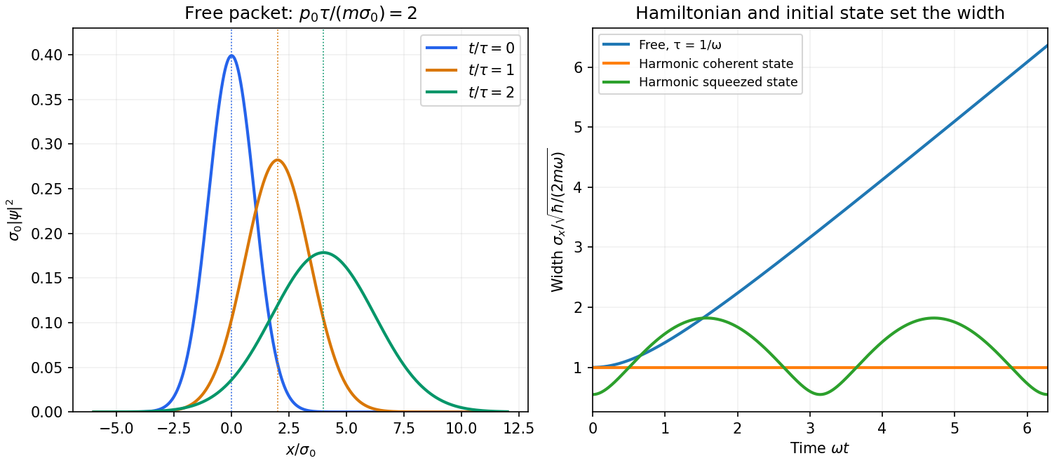


A potential energy changes this behavior. A quadratic potential preserves the Gaussian form because the evolution of position and momentum is linear. For a quantum harmonic oscillator, the Gaussian covariance in a harmonic potential isA coherent state has , and zero centered covariance. Its width is constant, and its center follows . In oscillator notation its coherent state label rotates as , apart from the common ground-energy phase of the state vector. A squeezed coherent state generally has a width that breathes at . Thus being Gaussian does not imply either free spreading or constant width; the Hamiltonian operator and initial covariance determine the result.
For a general nonquadratic potential, different parts of the packet experience different nonlinear forces, and an initially Gaussian profile need not remain Gaussian. Ehrenfest theorem gives the exact relations and . Replacing the last mean by is exact for a quadratic potential and approximate for a packet narrow compared with the scale on which the force varies. This connects packet motion to the correspondence principle without treating a quantum state as a definite classical path. Scattering can split a packet into reflected and transmitted components, while confinement can produce oscillations and interference between discrete energy eigenstates. Their relative phases evolve even when their populations remain constant. Localization, spreading and coherent motion all follow from the same linear unitary time evolution.