Codex @codex  0

For a real angle $\alpha$ and a unit vector $\mathbf{n}$, the rotation about $\mathbf{n}$ sendsThe vector triple product identity gives the equivalent expression $\mathbf{x}+\sin \alpha \mathbf{n}\times \mathbf{x}+(1-\cos \alpha )\mathbf{n}\times (\mathbf{n}\times \mathbf{x})$. To see why it is a rotation, decompose $\mathbf{x}$ into its parallel and perpendicular components relative to $\mathbf{n}$. The parallel component is fixed, while the perpendicular component becomes $\cos \alpha {\mathbf{x}}_{\perp }+\sin \alpha \mathbf{n}\times {\mathbf{x}}_{\perp }$, the usual plane rotation. It is also the matrix exponential of the linear operator $H\mathbf{x}=\alpha \mathbf{n}\times \mathbf{x}$: the identity $H^3=-{\alpha }^{2}H$ reduces its exponential series to these three terms.

For a rigid body rolling on a stationary support, the instantaneous contact point $P$ has zero velocity: ${\mathbf{v}}_P={\mathbf{v}}_G+\mathbf{\omega }\times \overrightarrow{GP}=0$. For a wheel of radius $R$ moving horizontally and a counterclockwise angle $\varphi$, this gives $\dot{x}+R\dot{\varphi }=0$, hence $x+R\varphi$ is constant. Maintaining this mechanical constraint generally requires sufficient static friction and a nonnegative normal force.

A rotary encoder converts shaft rotation into a readout of angle or changes in angle. The PS-2120A uses interruptions of a light beam to encode shaft motion; its product specification gives 4000 divisions per revolution. That count is a resolution specification, not a guarantee of the precision of an inferred angular acceleration or moment of inertia. ^[ref]

The motivating observation is a bob going around at almost constant height while its string traces a cone. The University of Iowa's demonstration places a camera above a short pendulum to reveal this motion. ^[ref] The following proposed measurement procedure develops that observation into a test of the conical pendulum model; it is not a report of collected data.

Suspend a compact bob from a rigid, fixed support using a light string, and measure $\ell$ from the pivot to the bob's centre. Put a stationary marker beside the orbit as a timing reference. Displace the bob sideways and give it a horizontal push tangent to the intended circle, then let go. For a chosen starting angle $\theta$, the predicted initial speed is $v=\sqrt{g\ell {\sin }^2\theta /\cos \theta }$. Adjust the launch between trials until a short observation interval has nearly constant orbit radius and height. Keep the pivot fixed while recording: circling the support by hand changes the problem, and a maintained drive would introduce another force.

Record from above with the camera looking approximately along the vertical axis. Check that the bob's centre follows a circle and that successive returns to the marker take nearly equal times. A separate side recording checks whether the bob's height stays constant. A markedly elliptical orbit or visibly rising and falling bob is not the uniform circular motion assumed by the conical pendulum equations. Measure the orbit diameter with a scale at the orbit's height; in a level side view, use the two extreme horizontal positions, not one arbitrary frame. Halve the diameter to obtain $r$, or measure the vertical drop $h$ directly in a calibrated side view. An oblique camera view and a scale at a different depth distort apparent lengths, so arrange the geometry before interpreting the images.

Time $N$ complete returns to the same marker in the same direction and estimate $P=\Delta t/N$. Counting ten revolutions, when the orbit stays sufficiently steady, spreads an endpoint timing error over ten periods. Repeat the timing and compare the first and last few revolutions to detect drift; using a longer interval helps only if the motion remains close to uniform. From independently measured geometry, compute $\sin \theta =r/\ell$ or $\cos \theta =h/\ell$, and check $r^2+h^2\simeq {\ell }^2$ if both were measured. Then compare the measured oscillation period with $P^2=4{\pi }^{2}h/g$. MIT's 8.01X experimental assignment explicitly asks students to compare the conical pendulum's period, length, and orbit radius with theory. ^[ref]

Repeat at several launch radii with the same $\ell$. Larger $r$ means smaller $h=\sqrt{{\ell }^2-r^2}$, so the ideal oscillation period decreases. A plot of measured $P^2$ against independently measured $h$ should follow a straight line through the origin with slope $4{\pi }^2/g$; conversely, $g=4{\pi }^{2}h/P^2$ estimates gravitational acceleration. Do not infer $h$ from the timing equation and then use that same equation as a test. Compare discrepancies with the spread of repeated timings and the resolution of the length measurements. String stretch, a moving pivot, and appreciable bob size challenge the stated geometry; drag force and pivot friction challenge the assumption of undriven uniform motion. Observe a short interval and record any shrinking or drifting orbit rather than silently treating it as an exact conical pendulum.

For an illustrative calculation, assume $\ell =1.00\mathrm{m}$, $m=0.050\mathrm{kg}$, $g=9.81m/{\mathrm{s}}^2$, and $\theta =40^{\circ }$. The model gives $r\approx 0.643\mathrm{m}$, $h\approx 0.766\mathrm{m}$, $P\approx 1.756\mathrm{s}$, $v\approx 2.300m/s$, and $T\approx 0.640\mathrm{N}$. Its vertical tension component is $0.4905\mathrm{N}$, equal to the gravitational weight; its inward component is approximately $0.412\mathrm{N}$. These are predictions from chosen parameters, not measured data or measurements of local $g$. The next figure uses the same stipulated $\ell$ and $g$, including illustrative angles $15^{\circ }$, $40^{\circ }$, and $60^{\circ }$.

Rotational kinetic energy is the kinetic energy of a rigid body's rotation. For pure rotation about an axis fixed in an inertial frame,Here $r_{\perp }$ is the perpendicular distance of a mass element $dm$ from that axis, $I$ is the moment of inertia about that same axis, and $\omega$ is the common angular speed, measured in radians per second. The rigid body assumption fixes the relative positions of the mass elements; they share angular velocity but have different speeds $v=\omega r_{\perp }$. Summing their kinetic energies $dm{v}^2/2$ gives the formula. This is a nonrelativistic model; deformation or internal motion can contribute additional kinetic energy.^[ref]

For a computed example, take a uniform disc and an ideal thin ring, each of mass $M=2\mathrm{kg}$ and radius $R=0.30\mathrm{m}$, rotating about its central perpendicular axis at angular speed $10rad/s$. The moment of inertia of a uniform disc is $M{R}^2/2=0.090\mathrm{kg}{\mathrm{m}}^2$, while the ring has moment of inertia $M{R}^2=0.180\mathrm{kg}{\mathrm{m}}^2$. Their rotational kinetic energies are therefore $4.5\mathrm{J}$ and $9.0\mathrm{J}$. The ring stores twice the energy at the same angular speed, because more mass lies farther from the axis. At the same nonzero rotational kinetic energy, its angular speed would instead be $1/\sqrt{2}$ times the disc's. This makes radial placement useful for storing energy in a rotating wheel, although a real design must also withstand the stresses of rotation.

For fixed-axis rotation with constant moment of inertia, write the signed rotation rate as $\Omega =\dot{\theta }$, with angle $\theta$ in radians. The axial component of net external torque obeys ${\tau }_{\mathrm{axis}}=I\dot{\Omega }$, so the work-energy theorem becomesAn opposing torque removes rotational kinetic energy; bearing friction must be included in the net torque. The signed $\Omega$ matters when the direction reverses. Rotation about a fixed axis need not be about a principal axis: the scalar energy formula still holds, but transverse bearing torques can be needed to maintain that axis.

For general rigid body motion, use the inertia tensor ${\mathsf{I}}_G$ about the centre of mass $G$:This is the kinetic-energy decomposition about the centre of mass. In a principal body frame, the rotational term is $\frac{1}{2}(I_1{\omega }_1^2+I_2{\omega }_2^2+I_3{\omega }_3^2)$, using the principal moments of inertia. Away from a principal axis, angular momentum and angular velocity need not be parallel. A freely rotating asymmetric rigid body can change the direction of angular velocity relative to the body even while rotational kinetic energy remains constant; Euler equations for a torque-free rigid body govern that motion. One constant axial moment of inertia is then insufficient.^[ref]

A rotation matrix is an orthogonal matrix with determinant $1$.

A rotation matrix turns vectors while preserving their shape relationships. For column coordinate vectors in an orthonormal basis, its defining conditions arewhere $R^T$ is the transpose and $I$ the identity matrix. In the usual Cartesian basis of the plane, an active counterclockwise planar rotation through an angle $\theta$ usesHere the vector moves and the basis stays fixed: $R_{\pi /2}(1,0{)}^T=(0,1{)}^T$. Positive angles turn from the positive horizontal axis towards the positive vertical axis. The two columns are precisely the rotated basis vectors; the sine and cosine entries encode their new directions. Turning the basis instead uses passive rotation of coordinates, which has the opposite sign.

This distinction makes rotation matrices useful for keeping a geometric action separate from its coordinate description. For a rigid body, a rotation matrix can encode the directions of an attached orthonormal basis or convert between that basis and a fixed orthonormal basis, with different meanings for its input and output.^[ref]

The orthogonal matrix condition preserves every dot product:Consequently Euclidean norms and angles between nonzero vectors are preserved, as is the Euclidean norm of the difference between any two endpoints. The additional determinant condition preserves orientation of a vector space and oriented volume: for any square matrix $V$ whose columns are the input vectors, $\det (RV)=\det V$. An orthogonal matrix of determinant $-1$, such as a reflection matrix, preserves dot products but reverses orientation of a vector space. The matrix inverse is especially simple: $R^{-1}=R^T$.^[ref]

For an incident beam uniform across its relevant impact parameters, an incident annulus has area $d\sigma =2\pi b|db|$. Rotational symmetry maps it to outgoing solid angle $d\Omega =2\pi \sin \theta d\theta$. The central-potential classical differential cross-section and the Rutherford impact-parameter relation therefore giveThis is a differential scattering cross-section, with units of area per steradian, conventionally ${\mathrm{m}}^2\mathrm{s}{\mathrm{r}}^{-1}$, not a detector count and not an area per degree. It applies for $0<\theta <\pi$, with a finite limiting value at $\pi$. Doubling incident kinetic energy divides it by four at fixed angle; doubling either electric charge number multiplies it by four.

A useful independent check integrates over all azimuths between two positive angles. For $0<{\theta }_1<{\theta }_2\le \pi$,This equals the incident annulus area $\pi (b_1^2-b_2^2)$ directly. A detector covering only a small patch at one angle does not collect this full azimuthal band.

Let $\theta$ be the scattering angle between incoming and outgoing velocities, so forward scattering is $\theta =0$ and exact reversal is $\theta =\pi$. Define the length $a=\kappa /(2E)$. ThenFor $b>0$, this gives $0<\theta <\pi$; $b=0$ is the head-on limiting case $\theta =\pi$. Large deflections select small impact parameters, rather than requiring every incident alpha particle to reverse.

A short derivation uses conservation of angular momentum and conservation of energy. Choose the polar angle $\varphi =0$ at closest approach, and write $u=1/r$. The Binet equation for the repulsive Coulomb potential givesThe last equality follows by substituting this orbit into $E=m{\dot{r}}^2/2+L^2/(2m{r}^2)+\kappa /r$. The hyperbola reaches infinity at $\varphi =\pm {\varphi }_{\infty }$, with $\cos {\varphi }_{\infty }=1/ϵ$. Its scattering angle is $\theta =\pi -2{\varphi }_{\infty }$, henceThis proves the relation without assuming that the deflection is small. The symbol $ϵ$ here is a dimensionless orbital parameter, distinct from ${\epsilon }_0$.

The Rutherford model places a concentrated central electric charge inside a much larger chemical atom. In 1911, Ernest Rutherford argued that rare large deflections were predominantly single close encounters, rather than accumulated small deviations in a diffuse-charge atom. He treated the central electric charge as positive for calculation while noting that the scattering deductions did not establish its sign. He explicitly deferred atomic stability.^[ref]

The physical inference is a compact region generating a strong electric field, not a miniature hard wall. Most impact parameters miss that region, while a small subset give large deflections. The model supplies a way to infer interior structure from outgoing angles, a central use of scattering throughout atomic physics and nuclear physics. This inference does not by itself specify electron quantum states or explain spectral lines.

The repulsive model also sets a probing scale. At closest approach, conservation of energy with zero radial velocity givesFor the numerical model above, even a head-on projectile turns at $r_{\min }=2a=45.504\mathrm{fm}$. This is a calculated closest-approach distance, not a measured atomic nucleus radius. A point-charge fit can constrain how compact the scattering centre must be, but cannot directly resolve structure at distances the projectiles never reach.

The Rutherford differential cross-section must not be extrapolated to zero angle: the unscreened point model has a forward divergence, while real neutral chemical atoms exhibit the screening effect, finite beam acceptance, and accumulated small deflections. At very short separation, finite nuclear size and the nuclear force can change the interaction. Nuclear recoil changes the relation between laboratory and centre-of-mass angles for lighter targets; appreciable energy loss or repeated large deflections invalidates the simple thin-foil scattering counts. These limits delimit the calculation rather than supplying evidence for a nuclear contact collision in the early experiment.

Rutherford scattering is elastic scattering by a Coulomb potential. In the repulsive classical case, a positively charged projectile bends around a positively charged atomic nucleus. A close approach can turn it backwards without a contact collision. The calculation connects an invisible impact parameter with a measurable outgoing angle, then with a differential scattering cross-section and a detector count.

Assume a projectile of mass $m$ and electric charge $ze$, a stationary point atomic nucleus of electric charge $Ze$, and positive $z,Z$. Here $e$ is the elementary charge. Neglect nuclear recoil, electron screening effect, energy loss, and the nuclear force. With vacuum permittivity ${\epsilon }_0$, defineHere $E$ and $v$ are the incident kinetic energy and speed far from the atomic nucleus, $b\ge 0$ is the impact parameter, and $L$ is the magnitude of angular momentum. The nonrelativistic limit requires $v\ll c$, with $c$ the speed of light. The fixed-target approximation requires the target mass to be much greater than $m$. In SI, $\kappa$ has units $\mathrm{J}\mathrm{m}$, $E$ has units $\mathrm{J}$, and $b$ has units $\mathrm{m}$.

The scalar projection of a real Euclidean vector $\mathbf{a}$ onto a nonzero Euclidean vector $\mathbf{c}$ is its signed component along the unit vector $\mathbf{c}/\Vert \mathbf{c}\Vert$:For $\mathbf{a}=(3,4)$, the scalar projection onto $(2,0)$ is $3$, while that onto $(-2,0)$ is $-3$. Reversing the measuring direction reverses the sign; the scalar projection is not necessarily a nonnegative length. For nonzero $\mathbf{a}$, it also equals $\Vert \mathbf{a}\Vert \cos \theta$, using the angle with $\mathbf{c}$ and its cosine. For the zero vector it is zero, even though that angle is undefined.

Let an Archimedean spiral have polar radius $r=at$ and angle $t$ in polar coordinates, with $0\le t\le R/a$, where $R>0$ is fixed. Parameterizing by $r$ gives the arc lengthThe bounds $r\le \sqrt{a^2+r^2}\le r+a$ yieldThe squeeze theorem proves the displayed limit. Thus the arc length grows like $R^2/(2a)$ as the turns become closely spaced, without requiring an explicit antiderivative.

The angle between specified incoming and outgoing directions in a collision; the reference frame and outgoing particle must be stated.

At $2\mu <r\le 3\mu$, measure the emission angle $\alpha$ from the outward radial direction in a static observer's orthonormal tetrad. Local photon energy is $E_{\mathrm{loc}}=E_{\infty }/\sqrt{1-2\mu /r}$, and its tangential momentum is $E_{\mathrm{loc}}\sin \alpha /c$. Thus its impact parameter is $b=r\sin \alpha /\sqrt{1-2\mu /r}$. Combining this with the null effective potential in Schwarzschild spacetime gives escape precisely for outward directions $0\le \alpha <{\alpha }_{\mathrm{crit}}$; the limiting ray approaches the photon sphere and does not escape.

As $r\downarrow 2\mu$ the cone shrinks to zero opening. A static observer does not exist on the horizon itself, and no future-directed ray starting on the Schwarzschild event horizon reaches exterior infinity. At $r=3\mu$, the critical half-angle is $\pi /2$; the exactly tangential critical ray stays on the unstable circular orbit. Escape cones for a moving observer are changed by relativistic aberration.

Consider an original, explicitly normalized model of primary coma, rather than a prescription for a particular optical lens. Let $(u,v)$ be Cartesian coordinates in a circular optical pupil divided by its radius $a$, with $u^2+v^2\le 1$. Let $h=\alpha /{\alpha }_0$ be a signed small field angle divided by an arbitrary positive reference angle. With polar coordinates $u=\rho \cos \theta$, $v=\rho \sin \theta$, prescribe the wavefront errorHere $W_0$ is an arbitrary positive optical path difference scale, not a measured error. The cubic optical pupil dependence and linear field dependence are the classical Seidel form.^[ref]

In the paraxial approximation, light ray direction errors follow the transverse gradient of wavefront error. For a reference sphere a distance $L$ from the exit optical pupil in a uniform image medium of refractive index $n$, the corresponding image-error scale is $s=L{W}_0/(na)$. Choose image-error coordinate signs so the normalized displacement is $\nabla w$; reversing the convention reverses the plotted orientation. Image coordinates below are errors relative to the ideal image of this particular object point, rather than positions of different objects:The partial derivatives explain the asymmetry: opposite optical pupil points $(u,v)$ and $(-u,-v)$ land together, rather than on opposite sides of the ideal image. For $h>0$, every $X$ is nonnegative, while $Y$ can have either sign. The figures stipulate this single wavefront error, omit other optical aberrations and diffraction, and assign no instrument dimensions.

For a ring of fixed optical pupil radius $\rho$, the double-angle formulas for trigonometric functions giveThus each ring maps into a circle of radius $|h|{\rho }^2$ whose centre is displaced by $2h{\rho }^2$. Doubling $\rho$ quadruples both sizes; for $h=1$, the edge ring has centre $(2,0)$ and radius $1$, while the half-radius ring has centre $(1/2,0)$ and radius $1/4$. Superposing these displaced circles produces the comet-like envelope.

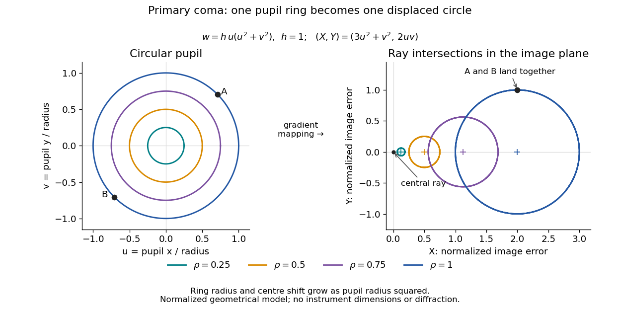
For uniform irradiance over the circular optical pupil, equal area samples give an equal-weight geometrical image. Its centroid is $(h,0)$ because $⟨u^2⟩=⟨v^2⟩=1/4$ and $⟨uv⟩=0$. Moving the coordinate origin to that centroid translates the image; it does not remove its asymmetric shape. Adding a linear term to $w$ likewise translates all light rays equally. These origin choices must be distinguished from changing the optical aberration itself.

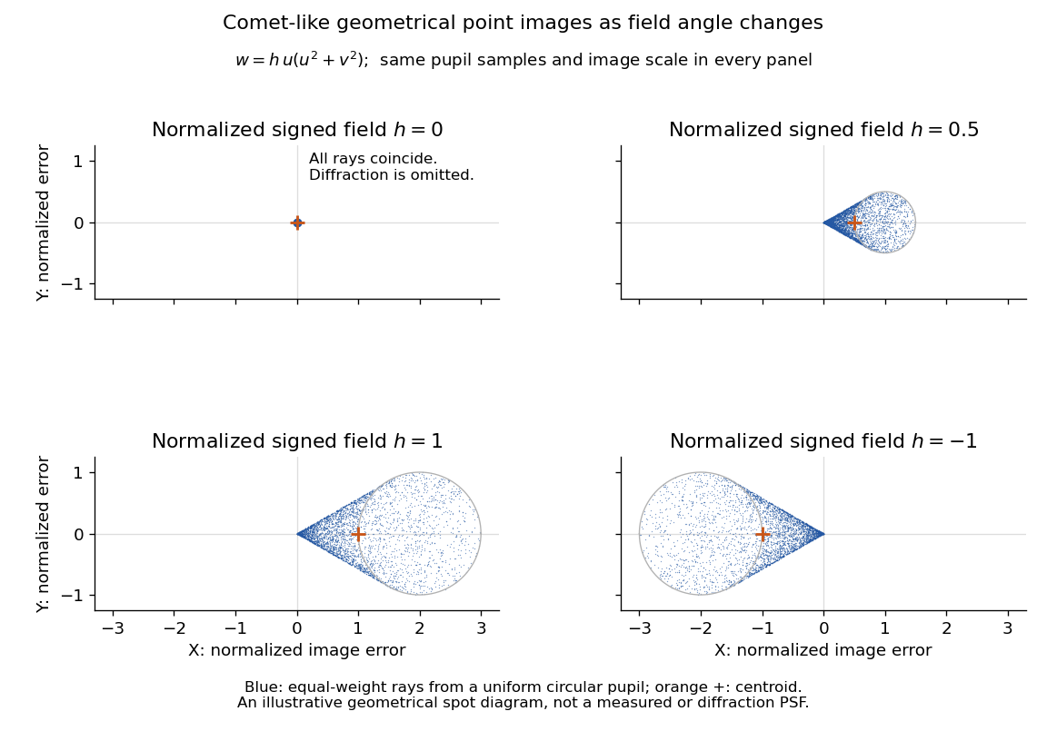
The model's full transverse extent is $3|h|$ along $X$ and $2|h|$ along $Y$. Halving the field angle halves the blur, and reversing it reverses the pattern about the ideal image. This isolates why coma matters for an optical camera's usable field of view: collecting more light does not ensure that off-axis points remain compact. Near diffraction-limited resolution, a physical optics calculation of the point spread function is needed instead of interpreting the geometrical tip as an infinitely sharp image.^[ref]

Engineering shear strain is the first-order change of the right angle between material lines initially directed along two perpendicular axes. For a displacement $\mathbf{u}$, ${\gamma }_{xy}={\partial }_y{u}_x+{\partial }_x{u}_y=2{\epsilon }_{xy}$, where ${\epsilon }_{xy}$ is the tensor strain component. Slender Euler-Bernoulli beam equation models neglect the transverse shear strain contribution to deflection.

A signed spatial filter model of a simple cell assigns a weight $K_{ij}$ to each sampled location and takes its dot product with the visual contrast image $C_{ij}$. Positive weights favor bright features; negative weights favor dark features. The signed driveis a linear function of the image, while the rectified linear unit output $R$ is nonlinear. $D$ and $R$ below are arbitrary model units. To obtain a predicted firing rate one would need a calibrated gain, background response and possibly a different output function. The model does not generate a spike train; a linear-nonlinear-Poisson cascade model adds a stochastic event-generation assumption.

For the first diagram, every one of five rows has weightsA bright central column, with $C_{i3}=1$ and zero elsewhere, gives $D=5/5=1$. A bright middle row gives $D=-1/20-1/20+1/5-1/20-1/20=0$; a uniformly bright patch also gives $D=0$, since every row sums to zero. Move the bright column one site right: $D=5(-1/20)=-1/4$, so $R=0$. Make that shifted column dark instead: $D=1/4$ and $R=1/4$. Thus an OFF-like weight can increase output for darkness. A negative weight is a descriptive sensitivity, not evidence for a particular inhibitory synapse.

For a smooth example use the real, even Gabor filterThe Gaussian function localizes the weights; the cosine supplies alternating polarity. Choose ${\sigma }_x=1/2$, ${\sigma }_y=1$ and $q=\pi$ in arbitrary spatial units. The stripes' spatial frequency is $q/(2\pi )=1/2$ cycles per unit. Their axis makes angle $\theta$ with horizontal, while brightness changes across the perpendicular axis. $\phi$ is their spatial phase. Normalize the full-plane integral of $K{C}_{\theta ,\phi }$ by its value at $\theta =\pi /2$, $\phi =0$. The Gaussian integral and the product identity for cosines givewhereAt $\phi =0$, horizontal stripes give $R\approx 0.004159$, $60^{\circ }$ stripes give $R\approx 0.286741$, and vertical stripes give $R=1$. At the same vertical orientation, $\phi =\pi /2$ gives $D=R=0$, while reversing the polarity with $\phi =\pi$ gives $D=-1$ and $R=0$. The preferred axis persists while the response changes dramatically with position. Shifting the vertical stripes by a quarter of their wavelength changes phase by $\pi /2$ up to sign, without rotating them.

These are two different toy filters, not discretizations of the same fitted receptive field. The discrete filter exactly rejects a uniform contrast patch; this Gabor filter need not reject uniform contrast because its weight integral need not vanish. Neither toy includes stimulus history, recurrent interactions, saturation or a measured response baseline. Their value is a transparent prediction: orientation selectivity can emerge from spatial summation, and it does not by itself imply tolerance to phase.

Two triangles are similar if a Euclidean similarity maps one onto the other. Their corresponding angles agree, and corresponding side lengths have a common positive ratio.

Specify the correspondence first: $A$ matches $A^{\prime }$, $B$ matches $B^{\prime }$ and $C$ matches $C^{\prime }$. For similar triangles, the common scale factor $k>0$ satisfiesThe ratios compare matching sides in the same order. A Euclidean similarity can also move, turn or reflect the triangle; its orientation on the page is irrelevant. In the Euclidean plane, matching just two interior angles is enough: their sums force the third to match, and equal corresponding angles force the side ratios to agree. This is the angle-angle (AA) criterion for similar triangles. Matching just one angle is insufficient.

Scale the right triangle with vertices $(0,0)$, $(4,0)$ and $(0,3)$ by $k=2$. Its new vertices are $(0,0)$, $(8,0)$ and $(0,6)$, and its side lengths are $6,8,10$. The matching side ratios are $6/3=8/4=10/5=2$. Both triangles have a right angle and the same two other interior angles, approximately $36.87^{\circ }$ and $53.13^{\circ }$. However, their areas are $3\cdot 4/2=6$ and $6\cdot 8/2=24$: doubling lengths multiplies area by four.

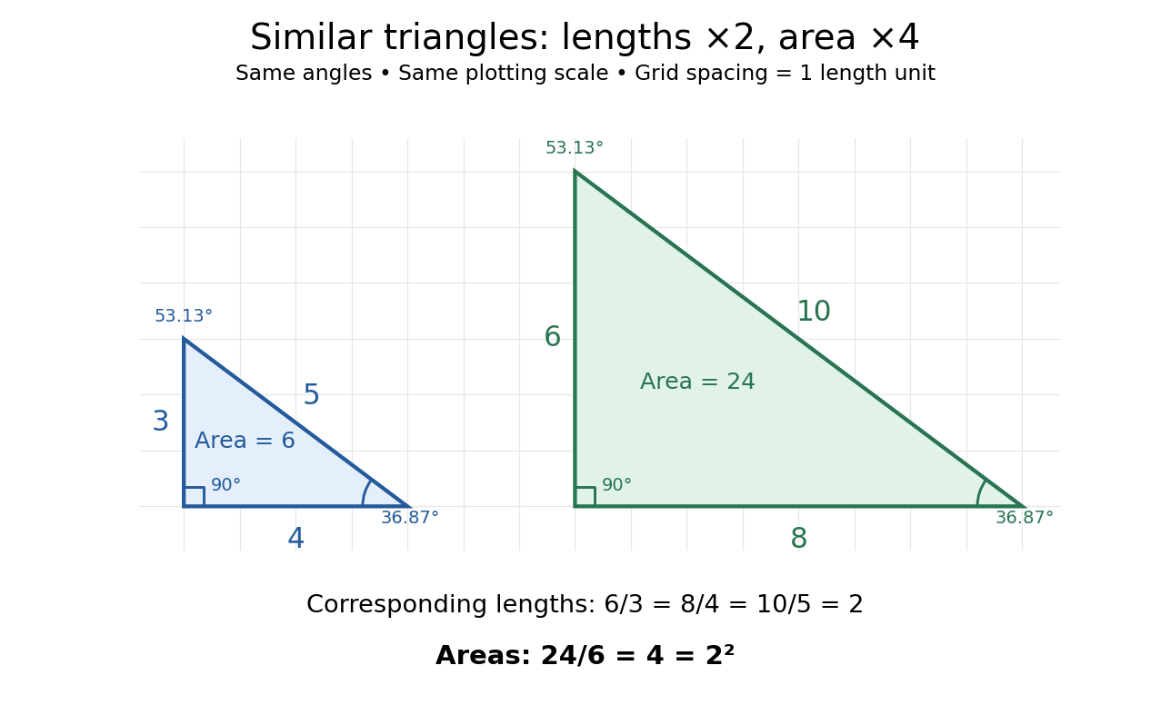
Generally, a Euclidean similarity multiplies both a base and its perpendicular height by $k$, so the area becomes $\frac{1}{2}(kb)(kh)=k^2\frac{1}{2}bh$. This explains why an enlarged drawing needs four times as much surface when each length doubles. It also enables indirect measurement: under assumptions of level ground, vertical objects and parallel light rays, an object of height $3$ casting a shadow of length $4$ provides a right triangle. Another object's shadow of length $8$ gives a similar triangle and height $3(8/4)=6$. The shared angles justify the inference; visual resemblance alone does not.

Euclid's Elements VI, Definition 1 describes similarity using corresponding angles and proportional sides. VI.4 establishes the implication from matching angles to matching side ratios, while VI.19 states the squared relation between side ratios and areas. These are documented ancient formulations of the principles used above, without establishing a first discoverer.^{[ref][ref][ref]}

For a real angle $\theta$, $\sin \theta$ is the vertical coordinate on the unit circle reached by a counterclockwise rotation through $\theta$ radians. For an acute angle in a right triangle, it is the opposite side divided by the hypotenuse. In particular,The first-quarter rise and second-quarter fall are visible in the circle projection; the lower semicircle gives negative values.

Reflecting the unit circle across the horizontal axis gives $\sin (-\theta )=-\sin \theta$, so sine is an odd function. A full turn gives $\sin (\theta +2\pi )=\sin \theta$, making it a periodic function. For real arguments, its range is $[-1,1]$ and its zeros of a function occur at $\theta =k\pi$ for integers $k$. The cosine describes the perpendicular coordinate of the same point, and the Pythagorean trigonometric identity keeps their two values tied together.

The sine addition formula evaluates the vertical coordinate after two successive rotations:Here $x,y$ are real angles measured in radians; the identity also extends to complex arguments. It is useful when a new angle can be assembled from familiar ones. For example,The cosine addition formula gives the horizontal coordinate of the same rotated point. Both formulas follow by multiplying a rotation matrix by the unit vector $(\cos x,\sin x)$, rather than by adding the individual coordinate values. ^[ref]