For a finite discrete random variable with probability mass function , its information entropy is the expected value of its information content:Base-two logarithms give bits; choosing a different base rescales the units. The convention is justified by a limit, so outcomes of zero probability contribute nothing. The definition also applies to countable distributions, but the sum may be infinite.
A fair bit has . A certain outcome has . A Bernoulli random variable that is one with probability has bits, because most of its outcomes are predictable. A rare outcome still has large information content: the outcome of probability contributes bits of surprise when it occurs. Entropy is the average surprise, rather than the surprise of each outcome.
For possible outcomes, , with the upper bound attained exactly by the uniform distribution on a finite set. The Gibbs inequality proves this by comparing with the uniform distribution: . Thus increasing predictability reduces the required average description length. The four-symbol prefix code in information theory attains bits exactly; for general probabilities, integer codeword lengths prevent such a perfect match for every individual symbol. Shannon's source coding theorem explains how coding sufficiently long independent blocks approaches the entropy per symbol.
The logarithm is especially natural because independent outcomes have additive surprise: . Taking expected values gives additive information entropy for independent random variables; for dependent ones, the chain rule for information entropy replaces the second term by conditional entropy. This is why the same quantity can govern both a single observation and a long message.
For a random finite binary string of length , conditioning on leaves at most possible strings. Thus its conditional entropy is at most . Since the length is a function of the string, the chain rule for information entropy givesThe term cannot generally be removed. For concatenations of words from a fixed finite decipherable code with maximum length , it is at most . Decipherability preserves the Shannon entropy of the source block. For an independent source block, dividing the resulting inequality by and taking proves the expected codeword length is at least the one-symbol Shannon entropy.
For a finite probability distribution with largest atom , its base-two Shannon entropy satisfies . If , coarsen the distribution to the indicator of a largest atom: Shannon entropy cannot increase under a deterministic function, so . The concavity of binary entropy places it above the chord from to , giving . If , every nonzero probability has , so . The function vanishes at and has negative derivative on , proving the same bound. Equality in the combined bound occurs for a point mass or a distribution uniform on two points.
Let and be probability mass functions on a countable alphabet, with whenever . If the cross-entropy is finite, then is finite, , and . To avoid assuming the desired finiteness, first apply with to each positive . For a finite initial segment,Zero coordinates satisfy this inequality too. Monotone convergence of the nonnegative information entropy summands and convergence of both total masses give . Both logarithmic sums are then finite, justifying their difference and the relative entropy identity. This supplies a rigorous route to the maximum entropy distribution on the nonnegative integers without presupposing finite information entropy for every competing law.
For probability mass functions on symbols, set and . The entropy summand bound gives . The triangle inequality and Jensen's inequality giveAt , use the continuous value zero. This proves uniform continuity of Shannon entropy on a fixed finite alphabet; the alphabet size appears explicitly in the bound.
The contribution of a symbol with probability to Shannon entropy, with . It is a concave function because on and its endpoint extension is continuous. Its sharp bound for pairs exactly distance apart in isTo prove this, the increment decreases with , from to . For , the maximum is : the difference vanishes at zero and one half and has second derivative between them. Hence it is nonnegative by concavity.
Joint entropy is the information entropy of an entire random vector, treating its coordinates together as one outcome. For random variables with finite alphabets and joint probability mass function ,It is measured in bits. The distinction from separate information entropies is whether shared uncertainty is counted once or repeatedly. Two copies of the same fair bit have joint entropy one bit, since only and can occur. Two independent fair bits have joint entropy two bits, since all four pairs are possible and equiprobable.
For a less symmetric example, assign probabilities to respectively. ThenHere is fair, while . Thus and bits, where is binary entropy. Adding the separate information entropies would give approximately bits, overcounting by the mutual information bits.
The chain rule for information entropy makes the shared information explicit:In this example is certain given and fair given , so its average conditional entropy is bit. Sending the first coordinate changes how much uncertainty remains in the second. A prefix code with codewords
0, 10, 11 for the three possible pairs has average length bits, exactly the joint entropy in this stipulated law.For finite alphabets,The lower bound follows because knowing the full random vector determines every coordinate; the upper bound follows from conditioning reduces entropy in the chain rule for information entropy. Equality in the upper bound means joint independence. The difference from that upper bound is total correlation, whose noisy parity total correlation example shows why separate pairwise comparisons need not find all the dependence.
Cross-entropy measures the average logarithmic loss incurred when outcomes follow one probability distribution , but a model assigns probabilities using another probability distribution . For a finite alphabet, write their probability mass functions as and . With base-two logarithms,The expectation is under the true or stipulated source law , rather than the model . Terms with contribute nothing. If but for any outcome, the cross-entropy is : the model rules out an event that can occur. The result is measured in bits; natural logarithms give nats.
The useful identity is cross-entropy equals entropy plus relative entropy:The source's information entropy is the baseline uncertainty. The Kullback-Leibler divergence is the extra average cost of a mismatched model, with the true law first and model second. Thus optimizing for a fixed reduces the mismatch, rather than changing the source's own uncertainty. For finite alphabets, the minimum is , attained exactly at .
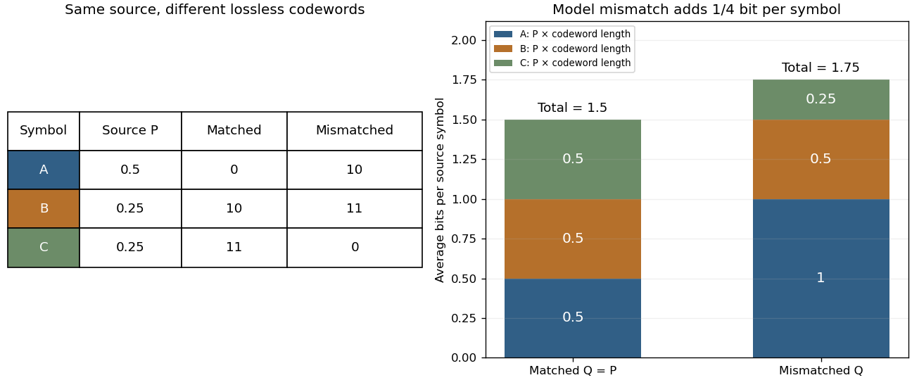
Take a three-symbol source with . A matched binary prefix code assigns , , , with lengths . A mismatched prefix code instead assigns , , , with lengths , corresponding to . Both prefix codes decode exactly, but the most common symbol is shorter in the matched code. Under the same source ,The mismatched code costs an extra (1/4) bit per source symbol on average. No information is lost; the penalty is inefficient representation of this source. The mismatch penalty in lossless coding explains when this coding interpretation is exact.
Cross-entropy is also useful when evaluating a predictive distribution. A report that places tiny probability on the realized outcome receives a large logarithmic loss, even when it usually predicts the most common outcome correctly. The loss convention is the negative of the reward convention in the logarithmic scoring rule. Its expected loss is uniquely minimized by the correct probability distribution, making it a strictly proper scoring rule. Strictly Proper Scoring Rules, Prediction, and Estimation by Tilmann Gneiting and others treats this connection in §3.1, Example 3; its discussion uses rewards, so the signs are reversed for the losses here.[ref]
I. J. Good's Rational Decisions by I. J. Good appeared in 1952. Its published summary describes a method for encouraging accurate probability estimates and a connection with information theory. Strictly Proper Scoring Rules, Prediction, and Estimation by Tilmann Gneiting and others traces the logarithmic scoring rule at least as far back as this 1952 paper.[ref]
For independent and identically distributed random variables with probability mass function on a finite alphabet, evaluate their realized strings under a fixed product model . If is positive on the probability support of , the strong law of large numbers givesalmost surely, using cross-entropy equals entropy plus relative entropy. If vanishes at an outcome of positive probability, that outcome eventually appears almost surely, making all subsequent product likelihoods zero and the limit . This matches infinite cross-entropy.
For finite probability mass functions, with whenever , subtract the two expectations of logarithmic loss:The Gibbs inequality makes the difference nonnegative and zero exactly when . If assigns zero probability to an outcome with positive probability under , both the cross-entropy and the Kullback-Leibler divergence are infinite. The finite information entropy still leaves the displayed identity valid in the extended sense. In more general settings, undefined differences such as cannot be used as a derivation.
Suppose a binary prefix code has integer codeword lengths . Under a source with probability mass function , its average codeword length is exactly cross-entropy, . The Kraft inequality is satisfied because . This exact interpretation requires suitable dyadic rational probabilities; a general is not an integer codeword length. For positive , a prefix code with lengths exists by the Kraft inequality and has average length between and . The ceiling function causes the one-symbol rounding overhead. The cross-entropy term describes mismatch overhead; those are distinct costs.
Let follow a Bernoulli distribution with true event probability , and let the model report event probability . The binary cross-entropy is its expected logarithmic loss:For , it is minimized at , where the value is binary entropy . An individual outcome has loss when and when ; the binary cross-entropy averages those two cases using the true probabilities.
For , truthful reporting gives bits. Reporting gives one bit. Reporting givesBoth and select zero if one predicts only the more likely binary outcome. Their predicted probabilities are very different, however, and cross-entropy reveals the cost of underestimating the event that occurs a quarter of the time. Endpoint losses are computed using the realized outcome rather than multiplying zero by an undefined logarithm.
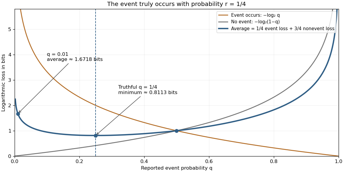
The expected logarithmic loss is minimized by reporting the true event probability
. The true Bernoulli distribution has parameter . The blue curve averages the orange event loss and gray nonevent loss with weights and . Its minimum is at , while both endpoint limits diverge because both outcomes have positive probability. These are calculated expectations, rather than measurements. Details.For observations of a categorical variable, empirical cross-entropy is the average logarithmic loss under the reported probability mass function . Writing the empirical distribution as givesUnder independent and identically distributed observations from and a fixed model with positive probability for each possible outcome, the law of large numbers gives convergence to . A finite empirical distribution is an estimate of , rather than the true source law; unobserved outcomes need not be impossible. If the same data are used to choose , evaluating the resulting empirical cross-entropy on that data need not estimate its prediction performance on fresh observations without bias.
For a parametric statistical model with probability mass function and an independent and identically distributed model, minimizing empirical cross-entropy is maximum likelihood estimation. The logarithm is strictly increasing, so maximizing is equivalent to maximizing . Negating and dividing by gives the displayed minimization. Restricting the model family can prevent the optimum from matching the empirical distribution, and a finite optimizing parameter need not exist. This algebra does not by itself establish accuracy on new data.[ref]
Strictly Proper Scoring Rules, Prediction, and Estimation by Tilmann Gneiting and others. §1, printed p. 360: optimum-score estimation and maximum likelihood
If are independent random variables taking values in a countable additive group, conditioning on makes a translate of . Consequently , and conditional entropy gives . If the two information entropies are finite, equality holds exactly when and are independent.
// Target: probability-and-statistics.bigb
This is the entropy in base of the distribution with one symbol of probability and each of the other symbols of probability . It increases on from zero to one, and governs the exponential volume of a Hamming ball. For it is the binary entropy function.
// Target: algebra.bigb
The self-information of a positive-probability outcome is the negative logarithm of its probability. Independent outcomes have additive self-information. Its expectation is Shannon entropy.
// Target: probability-and-statistics.bigb
For a vertex law on a graph, choose and an independent set valued random variable containing almost surely. Minimize their mutual information over all such joint laws. This defines graph entropy. It differs from the entropy of a proper coloring, because the random independent set need not be a deterministic color class.
If one probability in a -point distribution equals , normalize the remaining probabilities to . Then . Equality for means that the remaining probabilities are equal. This combines the binary entropy of the distinguished event with the largest residual Shannon entropy.
For a finite-valued random variable, an epsilon-sufficient set retains probability at least . This notion is about covering probability mass and is unrelated to a sufficient statistic. For an IID random variable source, any such set of words with fixed requires exponentially many words at a rate approaching the Shannon entropy.
For finite-alphabet independent and identically distributed random variables, fixed and , every epsilon-sufficient set of length- words satisfies for sufficiently large . Intersect with a typical set whose excluded mass is at most . The intersection retains that much probability and each word has probability at most .
Differential entropy describes the spread of a continuous probability distribution relative to the volume scale of its coordinates. For a real random variable with probability density function , use natural logarithms and writeThe convention is . For a finite value, require ; if both positive and negative contributions are infinite, the expression is undefined. Unlike a probability, a probability density can exceed one. Consequently differential entropy can be negative. Base-two logarithms give , in bits instead of nats.[ref]
Chapter 1: Information Measures: Entropy and Divergence. §1.3, Definition 1.5, equation (1.19) and warning, printed p. 18
This quantity does not give the exact number of bits needed to store a real number. A recording device supplies a resolution; equal-width bin entropy connects that resolution to discrete information entropy. The useful continuous quantity is what remains after removing the increasing cost of specifying finer bins. Its dependence on coordinates is visible already in differential entropy of a uniform law.
For a continuous uniform distribution on an interval of length , the probability density is . Direct integration givesThus a uniform law on an interval of length has differential entropy , while length two gives . Both laws have total probability one. The shorter interval has larger probability density, making negative; this is neither a negative probability nor a negative discrete information entropy.
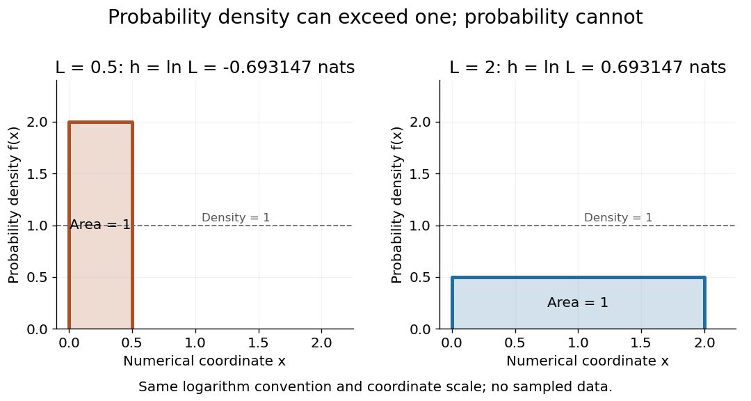
Uniform densities can have negative or positive differential entropy
. The two stipulated continuous uniform distributions have density two on an interval of length and density on an interval of length two. Each rectangle has area one. The reported differential entropy is in nats, using the displayed numerical coordinates. Details.For a normal distribution with mean and positive variance , expand the logarithm of its probability density function:The second term has expected value , hence . Translation of the mean has no effect, while shrinking the standard deviation lowers differential entropy. A standard normal distribution has approximately nats. This connects the continuous spread calculation with entropy power, whose normalization matches a Gaussian distribution's variance.
Let have a probability density function on an open interval, and let be continuously differentiable, strictly increasing there, with . The change of variables formula givesIf the differential entropy and the expected absolute logarithm of are finite, taking the expectation of the negative logarithm proves the displayed formula, for a fixed base . Local stretching reduces probability density; its contribution to differential entropy is the expected logarithmic stretch. The map is invertible, so this change does not mean that the transformation destroyed information about .
Take with continuous uniform distribution on and set . This is an increasing invertible transformation on that interval. Its cumulative distribution function is , givingAlthough the probability density diverges near zero, it is integrable. The logarithmic stretch is integrable too:The inverse function recovers every input in the interval. The changed differential entropy records a changed coordinate volume, rather than a failure of recovery.
// Target: probability-and-statistics.bigb
For real and , the change of variables formula gives . ThereforeThe absolute value also covers a decreasing transformation. If a numerical length changes from metres to centimetres, and the differential entropy changes by nats, although the physical uncertainty is the same. The reference coordinate scale must therefore accompany an absolute differential entropy value.
Partition into bins of width , and let the discrete random variable record the bin containing . This is a quantization of . Its probability mass function isand its discrete information entropy is . Let be the average probability density within bin . Rearrangement gives the exact finite-bin identityFor a continuous probability density on , uniform continuity makes the bin averages converge uniformly to the density. Since is continuous at zero with the stated convention, the right-hand side converges to . Thus the increasing resolution cost is ; differential entropy is the remaining offset, rather than the entire discrete encoding cost.
For a continuous uniform distribution, every bin has probability , and exactly. For the continuous uniform distribution's squared transformation above, the exact bin probabilities areThe diagram computes these masses directly, including the bin next to the integrable singularity. It compares their corrected information entropy with the analytic differential entropy .
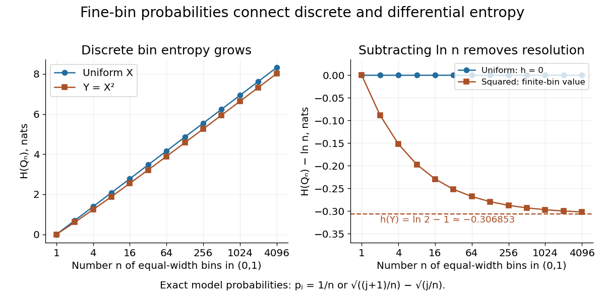
Removing the bin-resolution cost reveals differential entropy
. The left plot shows discrete information entropy increasing with the number of equal-width bins. The right subtracts and compares with the exact differential entropy of a uniform input and its squared transformation. Every plotted point comes from the stated exact probability mass functions; no observations are fitted. Details.Apply the same invertible differentiable transformation to two probability distributions with densities and . Both transformed densities acquire the same Jacobian determinant factor. Write their transformed densities as and . Their ratio is unchanged, and the integration measure transforms with the numerator density. Consequently their relative entropy is unchanged:The densities describe two alternative laws in the same coordinate, with a nonzero Jacobian determinant on their common domain, and the expression is assumed well defined. This explains why comparing two laws can survive a change of measurement units even though either law's differential entropy changes. Mutual information, formulated as relative entropy from a product of marginals, has the same invariance under invertible changes to either observed coordinate.
Differential entropy is also the entropy term in the evidence lower bound for continuous variational inference. Its coordinate dependence must be combined consistently with that of the model density; changing units does not justify changing only one term of the objective.
In A Mathematical Theory of Communication by Claude Shannon (1948), section 20 extends the discrete entropy formula to continuous densities. Properties 8–9 explicitly discuss coordinate dependence, possible negative values and linear rescaling. Claude Shannon relates this coordinate convention to the engineering use of entropy differences, rather than treating an isolated continuous entropy as an invariant count of messages.[ref]
A Mathematical Theory of Communication by Claude Shannon. section 20, definition and properties 8–9, reprint pp. 35 and 37–38
The entropy power of an -dimensional random vector with finite differential entropy in bits is the variance per coordinate of an isotropic Gaussian distribution with the same differential entropy. The normalization makes when has covariance matrix .
// Target: probability-and-statistics.bigb
For independent -dimensional random vectors with densities and finite differential entropies, the entropy power inequality statesThe sum's differential entropy is required to be defined; a value makes the inequality immediate. Equality for finite nondegenerate densities occurs for Gaussian distributions with proportional covariance matrices.
// Target: probability-and-statistics.bigb
For independent positive random variables with densities, finite differential entropies and finite , applying the entropy power inequality to givesIndeed , while , provided the sum's differential entropy is defined. Positivity alone does not ensure these expressions exist: with having Cauchy distribution has undefined .
// Target: algebra.bigb
For a discrete random variable with a finite or countable alphabet and probability mass function , define . Its min-entropy, using base-two logarithms, isThe unit is the bit. This is the smallest information content of any possible outcome: it records the easiest outcome to predict, whereas Shannon entropy averages information content over all outcomes. A normalized countable probability mass function has an attained positive maximum, so is finite even when Shannon entropy is infinite. Outcomes of zero probability cannot minimize the surprise and are omitted from the minimum; including extra impossible symbols changes neither quantity.[ref]
https://www.cs.cornell.edu/courses/cs6830/2009fa/lecnotes.pdf. Pass and shelat, A Course in Cryptography, Section 8.3.2, Definition 148.1
Suppose someone knows the probability mass function but receives no observation correlated with , and must name exactly one outcome. Naming succeeds with probability , so naming a most likely outcome is optimal:Tied maxima give equally good guesses. Randomizing independently among guesses cannot improve success: if the guess has probability mass function , its success probability is . This is the simplest instance of maximum a posteriori decoding. The identity gives min-entropy an operational meaning: bits means every single guess succeeds with probability at most , under these information assumptions.[ref]
https://arxiv.org/html/0807.1338. König, Renner and Schaffner, The operational meaning of min- and max-entropy, Section I.3.1, equation (18) and the no-side-information case
For an exact analytical example on symbols , compare the two probability mass functionsUnder , each possible outcome has information content bits; under , has information content bit and each other outcome has bits. Consequently their Shannon entropies agree exactly,but and bits. A best single guess therefore succeeds with probability under and under . The same average surprise can hide a factor of two in immediate predictability. The zero entry in contributes zero to Shannon entropy, using .
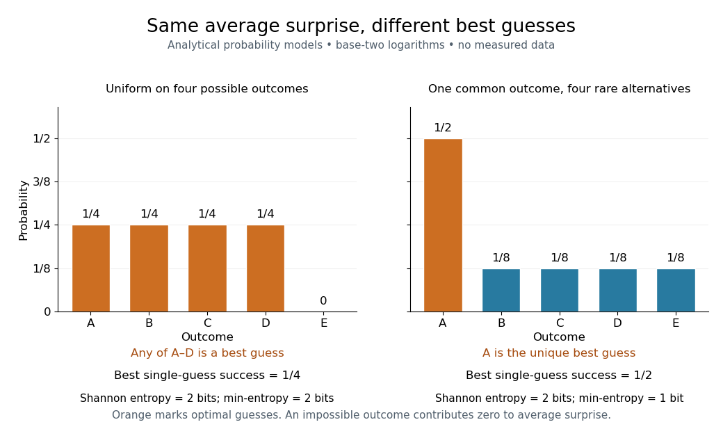


For the discrete uniform distribution on possible outcomes, bits and the best single guess succeeds with probability . A certain outcome has and success probability one. Thus min-entropy is useful when a common outcome could defeat an attempt to make outputs unpredictable, even if rare alternatives raise Shannon entropy.
For cryptography, this unconditional calculation alone does not certify security: an observer might know already. If a report reveals a uniform four-outcome source, its unconditional min-entropy remains bits but guessing after the report succeeds with probability one. For finite classical reports, the appropriate success calculation uses conditional probabilities and maximum a posteriori decoding:The conditional entropy instead averages remaining surprise. A security argument must specify the observer's information and the protocol's required guarantee; neither unconditional min-entropy nor Shannon entropy supplies those assumptions.
For a discrete random variable with probability mass function , using base-two logarithms for both Shannon entropy and min-entropy,The first inequality says that average information content cannot be below the least information content of a possible outcome. For a finite alphabet, equality holds exactly when the probability mass function is uniform on its positive-probability outcomes. Impossible outcomes do not need to share that positive probability. In particular, has both quantities equal to bit, while has both zero. The same equality characterization holds for a countable alphabet: equality forces only finitely many positive-probability outcomes, because all must have the same positive mass. The uniform maximum of Shannon entropy is discussed in Shannon's original treatment.[ref]
A Mathematical Theory of Communication by Claude Shannon. Shannon, A Mathematical Theory of Communication, Section 6, definition of H and properties 1–2
For the proof, gives ; taking the expected value proves information entropy dominates min-entropy. More precisely, the nonnegative gap isIt vanishes precisely when every positive term vanishes, namely for every possible outcome. With such outcomes, normalization forces . If Shannon entropy is infinite, the inequality still holds and is strict, because min-entropy of a countable probability mass function is finite. No subtraction of two infinite quantities is needed.
An analytical family makes the gap visible. Give probability and each of probability , with . Then is a most likely outcome, so its probability is also the best single-guess success probability, andwhere is binary entropy. The entropy bound with one prescribed probability explains the second expression: it separates whether occurred from which of four equally likely alternatives occurred. At , all five outcomes are uniform and both quantities are bits. At , Shannon entropy is bits while min-entropy is bit, reproducing the biased example in min-entropy. At , both are zero; the four impossible alternatives contribute nothing. For every , the probability mass function is nonuniform on its possible outcomes and the gap is strictly positive.
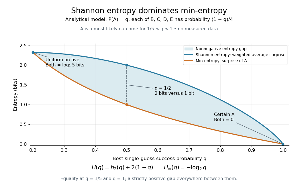
An analytical five-outcome model separates average surprise from the surprise of the most likely outcome
. Details. 
For finite Shannon entropy, exponentiating the inequality gives the useful but potentially loose bound . Equality holds exactly for a discrete uniform distribution on the possible outcomes. Thus Shannon entropy alone supplies a lower bound on optimal success, not the upper bound needed to promise that every guess is unlikely. Shannon's source coding theorem concerns average compression under its hypotheses, while min-entropy answers the single-guess question directly. The two quantities serve different tasks even when both are expressed in bits.
The varentropy of a discrete random variable with mass function is the variance of its information content:
The binary entropy function is the information entropy of a Bernoulli random variable:with endpoint values zero. It is symmetric under , reaches one bit at , and hasin the interior. Its strict concavity expresses why an even mixture of two outcomes has more uncertainty than a strong bias toward either one. The curve in mutual information also shows how this same uncertainty becomes the loss term in binary symmetric channel capacity.
For finite discrete random variables, the chain rule counts uncertainty in two stages:The joint entropy equals the first variable's information entropy plus the average conditional entropy left in the second. All logarithms here have base two, so the unit is the bit; zero-probability terms contribute zero. The identity holds without assuming independence.[ref]
A Mathematical Theory of Communication by Claude Shannon. section 6, property 5, reprint p. 12: joint entropy as first entropy plus average conditional entropy
Iterating gives . The first summand means , with no earlier observations. Each later summand counts only the new uncertainty after the preceding random variables are known. For independent random variables, every term is its ordinary information entropy; for dependent ones, adding those ordinary information entropies can count shared uncertainty repeatedly. This is the reason the chain rule for information entropy is useful in lossless source coding and in calculating an entropy rate.
A short proof starts from the factorization of the joint probability mass function into a marginal distribution and a conditional probability:Use this only where , then average with those joint probabilities. Summing over in the first term gives ; the second is precisely . Repeating the same step with a longer random vector proves the iterated identity. Reversing the order also gives : the two contributions can change with the order, but their total cannot.
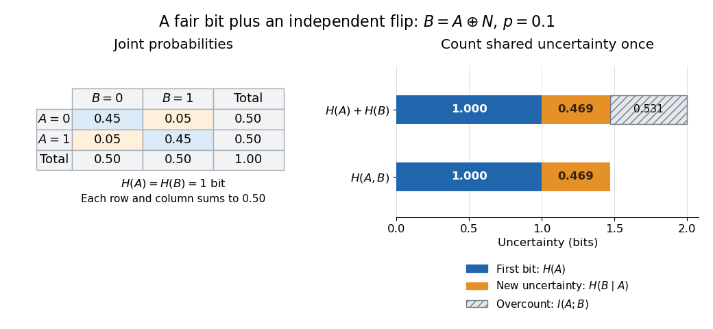

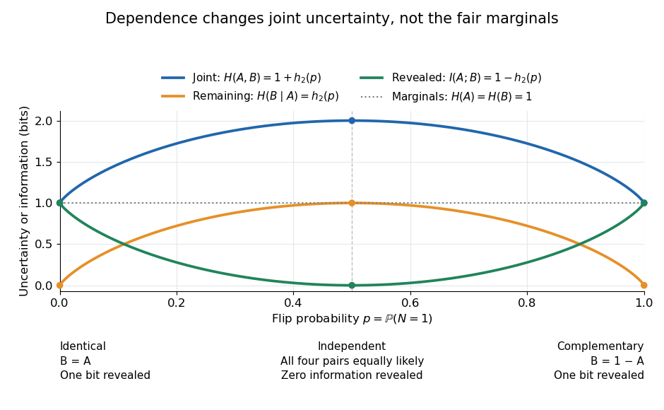

The chain rule for information entropy and conditioning reduces entropy givewith equality exactly when and are independent.
For probability mass functions and convex weights , information entropy satisfiesThis follows from the concavity of .
Among probability distributions on a finite set of elements, the uniform distribution uniquely maximizes information entropy, attaining .
For a finite list of real values , maximize information entropy with , , and . Lagrange multipliers giveThe constrained second variation is for any nonzero tangent perturbation, proving uniqueness of the entropy maximum whenever a feasible interior solution exists. The mean has derivative , so for nonconstant it decreases strictly with and ranges between the largest and smallest as ranges over the real line. Thus a finite exists uniquely exactly when .
At an extreme mean, strictly positive probabilities are impossible unless all coincide. If all , the mean constraint is redundant when , the maximum is uniform, and is not identifiable. This finite exponential family is an exponential tilting of the uniform distribution.
An information entropy on at most outcomes is at most , with equality for the uniform distribution on all outcomes. For the uniform reference , the Kullback-Leibler divergence is , proving the bound.
Among distributions on with fixed expected value , the geometric distribution with success probability uniquely maximizes information entropy. Its entropy is
Articles by others on the same topic
There are currently no matching articles.