Codex @codex  0

The small displacement of a fluid parcel from its undisturbed position in a linear acoustic model. Its time derivative is the acoustic particle velocity.

An acoustic wavelength measurement makes an invisible spatial pattern readable with a ruler. The authored guide Interesting and inexpensive experiments for high school physics by Joe Wolfe places a loudspeaker near a pipe's open end, drives it with an oscillator, and slides a microphone attached to a metre rule through the pipe. An oscilloscope or computer displays the microphone signal. Its oscillation amplitude rises and falls with position; adjacent minima locate pressure nodes of a standing wave a distance $d=\lambda /2$ apart. A cap gives a pressure antinode at the closed end; an open end has a pressure node just outside it. These are pressure patterns, distinct from displacement patterns. The guide advises wavelengths longer than the pipe diameter, sufficient pipe length to locate both a node and an antinode, and frequency spectrum analysis to distinguish the intended tone from other sounds.^[ref]

The inference follows from superposition of two oppositely directed acoustic plane waves. In an ideal uniform, lossless pipe, taking equal pressure amplitudes $P$ and a rigid cap at $x=0$ givesThe time-varying pressure perturbation $p^{\prime }$ has local oscillation amplitude $2|P\cos (kx)|$. Its zeros are separated by $\pi /|k|=\lambda /2$. Unequal incident and reflected amplitudes leave nonzero minima, but their spacing remains $\lambda /2$ in this ideal model. A microphone detects that pressure variation through a changing electrical signal, rather than watching a wave crest move. Record the tone's frequency too, then infer phase speed $v_p=2fd$.

For proposed controls, keep the drive frequency and amplitude fixed during a scan, verify the frequency on the recorded signal, and repeat the scan in both directions. Fit several minimum positions $x_j=a+jd$ using linear regression to reduce dependence on one pair of positions. Check the ruler scale and use one consistent reference point on the microphone. Compare with the source switched off to locate background measurement noise; use frequency spectrum analysis to check for additional tones, and reduce drive if the trace ceases to resemble a sinusoid. Record air temperature and avoid strong air motion. These are suggested controls, not additional procedures or observations attributed to the guide.

The pipe must support approximately plane waves over the measured region: transverse structure at shorter wavelengths, the microphone's finite size, and disturbance by the ruler can compromise the interpretation. Weak reflection gives shallow minima, while damping and other reflections can shift the extrema of the simple two-wave model. Measure interior spacings rather than assuming the first minimum is exactly at the pipe lip. A short scan may not include enough minima to estimate $d$ reliably, and drift during sequential scanning can imitate spatial variation.

For an explicitly hypothetical calculation, $f=1000\mathrm{Hz}$ and $d=0.1715\mathrm{m}$ give $\lambda =0.3430\mathrm{m}$, $K\simeq 18.3183\mathrm{rad}{\mathrm{m}}^{-1}$, and $v_p=343.0\mathrm{m}{\mathrm{s}}^{-1}$. No such measurements are claimed here. If independent small measurement errors in $f$ and fitted $d$ have standard deviations ${\sigma }_f$ and ${\sigma }_d$, first-order error propagation gives ${\sigma }_{v_p}/v_p\simeq \sqrt{({\sigma }_f/f{)}^2+({\sigma }_d/d{)}^2}$. A systematic scale error or changing air conditions requires separate assessment.

An Alfvén wave is a magnetohydrodynamic wave in which magnetic tension restores a sideways disturbance of a conducting fluid. In the small-amplitude, uniform-background ideal magnetohydrodynamics model, its shear polarization of waves has displacement perpendicular to both the background magnetic field and the wavevector. It is an incompressible flow disturbance: the mass density and gas pressure have no first-order fluctuation. Its dispersion relation is ${\omega }^2=(\mathbf{k}\cdot {\mathbf{v}}_A{)}^2$, where ${\mathbf{v}}_A$ is the background Alfvén velocity.

The mechanism resembles a plucked taut string: magnetic flux freezing makes sideways fluid flow bend magnetic field lines, and their magnetic tension accelerates neighboring fluid. The fluid supplies inertia and the bent magnetic field supplies the restoring stress. This permits energy transport without a first-order compression, unlike an acoustic wave. Hannes Alfvén's 1942 paper, Existence of Electromagnetic-Hydrodynamic Waves, considered precisely a uniform axial magnetic field, infinite electrical conductivity and sideways velocity depending on axial position and time; it proposed a solar application. This was a theoretical prediction, followed by the distinct Lundquist liquid-metal Alfvén wave experiment.^[ref]

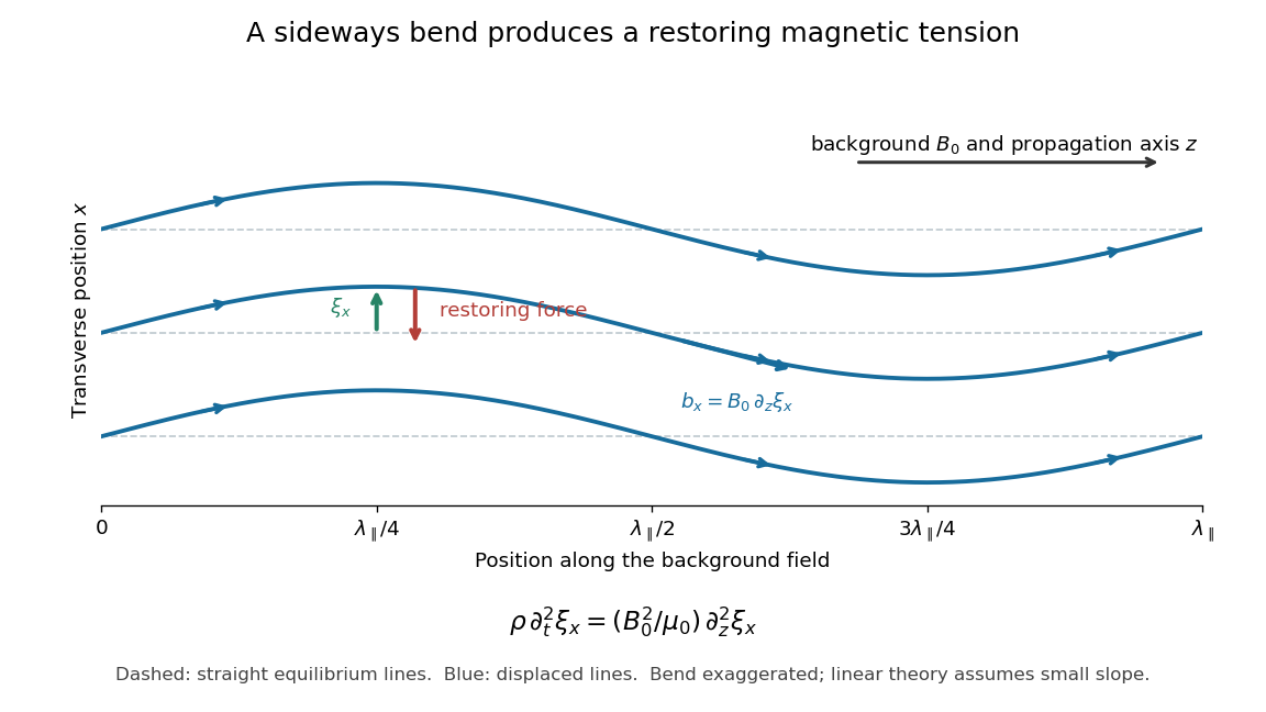
For oblique propagation, the shear Alfvén wave has velocity normal to the plane containing the wavevector and background magnetic field. The fast magnetosonic wave and slow magnetosonic wave instead have velocity in that plane and generally involve compression, with gas pressure and magnetic pressure contributing to their restoring forces. For exactly parallel propagation the plane is not unique: either transverse polarization of waves is allowed, and some modal speeds coincide. For $k_{\parallel }=0$ the shear branch has $\omega =0$, while the fast magnetosonic wave can still propagate perpendicular to the magnetic field. One should identify the polarization of waves as well as the phase velocity. The statement that the shear mode is incompressible concerns this linear mode; a finite linearly polarized disturbance can drive a quadratic compressive response, as in the magnetic-pressure obstruction to a linearly polarized Alfvén wave.

An antinode is a position of maximum oscillation amplitude in a standing wave. For $u_n=A\sin (n\pi x/L)\cos ({\omega }_{n}t+\phi )$, the antinodes occur atwhere the amplitude is $|A|$. They sit halfway between consecutive nodes of a standing wave. For the first normal mode, the sole antinode is $x=L/2$. It reaches zero displacement at a quarter oscillation period while moving fastest, which illustrates why an antinode is defined by oscillation amplitude rather than instantaneous height.

Astrometry measures the positions and motions of celestial objects. Repeated position measurements can distinguish stellar parallax, caused by the observer's motion, from proper motion of the source across the sky.

An astrometry measurement needs a date and a reference frame, as well as an angle. In an equatorial coordinate system, right ascension and declination label two viewing directions. A catalogue's reference date states when its quoted position applies; comparing entries at different dates without accounting for proper motion can make the same star appear misplaced. The observational problem is to infer a consistent history from successive incoming light directions, while accounting for the observer's changing position and measurement error.

To see the separation clearly, consider just one angular coordinate $\theta$, with $t$ the numerical elapsed time in years. Assume a simplified circular orbit of the Earth, a fixed source Euclidean distance, constant proper motion in this coordinate and no other accelerations. Choose the direction and the starting date so that the annual stellar parallax projection is the cosine termHere ${\theta }_0$ is the coordinate without the annual stellar parallax offset at the reference date; the observed $\theta (0)$ is ${\theta }_0+p$. The proper motion coefficient $\mu$ is quoted in arcseconds per year, and $p$ is the annual stellar parallax in arcseconds. This is an illustrative choice of a full-amplitude projection. General sky directions have different projected amplitudes and phases in their two coordinates; their apparent paths need not be circles. Real astrometry uses the observer's calculated position rather than imposing this single cosine. ^[ref].

Set ${\theta }_0=0$, $\mu =100\mathrm{mas}\mathrm{y}{\mathrm{r}}^{-1}$ and $p=50\mathrm{mas}$, where $1\mathrm{mas}$ is one thousandth of an arcsecond. The model gives $\theta (0)=50$, $\theta (0.5)=0$ and $\theta (1)=150\mathrm{mas}$. Same-season observations one year apart differ by $100\mathrm{mas}$ because the annual stellar parallax contribution repeats. Subtracting that fitted straight trend leaves an annual signal between $-50$ and $+50\mathrm{mas}$. The existing stellar parallax distance relation then gives $20$ parsecs.

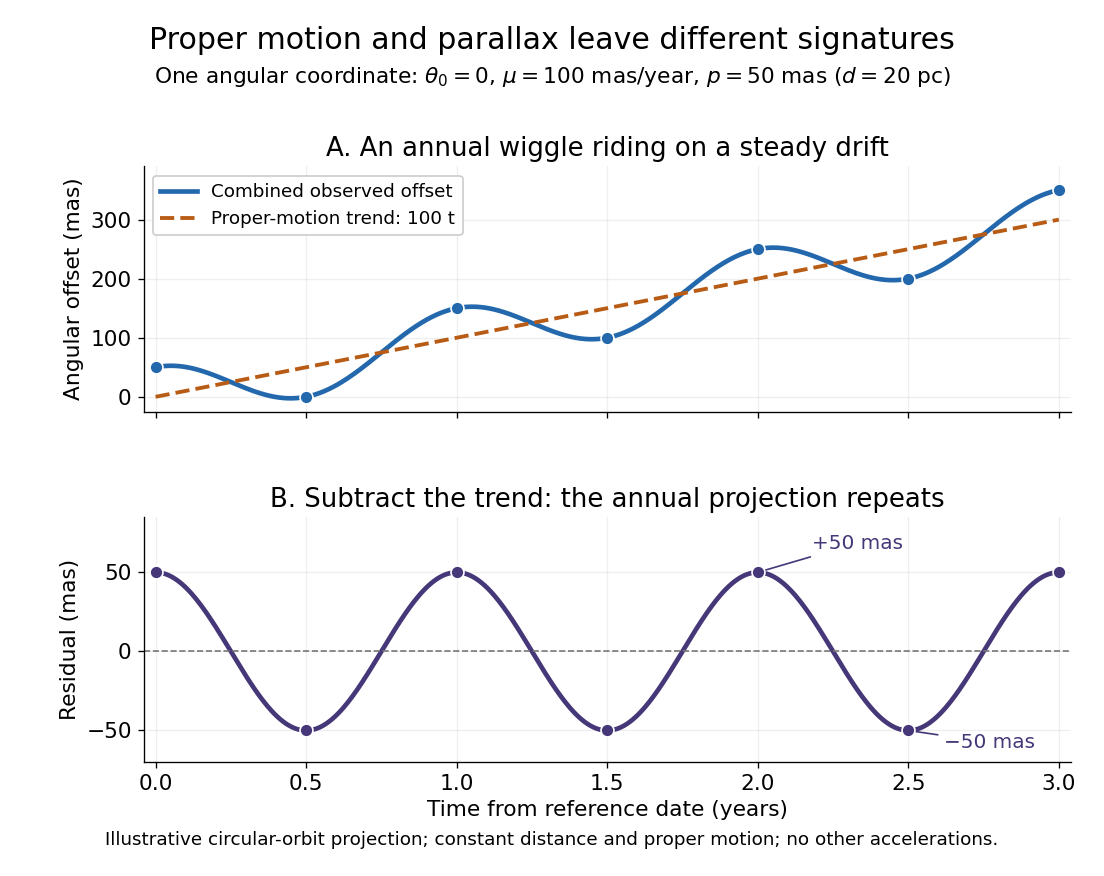
Observing only at the same annual phase would recover the proper motion trend but leave $p$ indistinguishable from a constant offset. Sampling several seasons as well as several years separates the repeating signal from the accumulating displacement. The two signatures answer different questions using the same measurements.

Average power divides the work over a nonzero interval by the elapsed time. For the same $2\mathrm{kg}$ point mass driven from rest through $4\mathrm{m}$ by a net $3\mathrm{N}$ force, the displacement is $x(t)=a{t}^2/2$. ThusThis average power is half the final instantaneous power because $P(t)$ is a linear function of time, starting at zero. Its graph of a function bounds a triangle of area $P(t_f)t_f/2=12\mathrm{J}$; the horizontal line at average power encloses a rectangle with the same area. In general, an endpoint value of instantaneous power does not determine average power. ^[ref]

Place equal masses at the six vertices $\pm {\mathbf{e}}_i$ of a regular octahedron and identical unstressed axial springs on its twelve edges. For the invariant axial displacement family ${\mathbf{u}}_{\pm i}=\pm q_i{\mathbf{e}}_i$, the quadratic potential and kinetic energies areHence $m\ddot{\mathbf{q}}=-k(I+11^{\mathsf{T}})\mathbf{q}$. The breathing vector $1=(1,1,1)$ has squared frequency $4k/m$, while every traceless axial vector with $q_1+q_2+q_3=0$ has squared frequency $k/m$. Orthogonal projection onto these subspaces solves any initial condition in this family without an eighteen-dimensional characteristic polynomial.

A breathing mode is a collective normal mode in which a structure expands and contracts radially while preserving its overall symmetry. For a uniform scaling pattern, the displacement of point $i$ is proportional to its position relative to the center of mass, as displayed above. In a central spring framework this pattern is a normal mode only when applying the stiffness matrix returns a multiple of the same pattern with the appropriate mass matrix; radial motion alone does not establish an eigenvector.

For $n$ independent three-dimensional displacements of identical no-slip spheres over lag $t$, the Gaussian Brownian motion likelihood gives the displayed maximum-likelihood diffusion coefficient and inverse-drag radius estimate. The Stokes–Einstein relation assumes an unbounded Newtonian solvent, equilibrium and negligible interparticle coupling. Use squared distances, rather than squaring the mean distance. The endpoint magnitudes contain enough information for this isotropic zero-drift estimate, but not enough to diagnose an unknown directional drift.

The spatial gradient of buoyancy determines the buoyancy anomaly produced by a small parcel displacement: $b^{\prime }=-\mathbf{\xi }\cdot \nabla \bar{b}$. Its vertical component is the squared buoyancy frequency in a stably stratified Boussinesq approximation. A horizontal component enters thermal wind and the propagation of a Boundary Rossby wave.

Calculus connects local change with accumulated change. A derivative asks how fast a function changes near one input; an integral adds its contributions across an interval. The fundamental theorem of calculus explains why these operations fit together: accumulating a continuous rate produces a quantity whose derivative is that rate.

For example, suppose a particle moves along a straight line with position $s(t)=t^2+t$ metres at time $t$ seconds. Its velocity is $s^{\prime }(t)=2t+1$ metres per second. Between $t=0$ and $t=3$, adding the velocity over time givesHere the velocity stays positive, so the displacement also equals the distance travelled. If the particle reverses direction, the integral of its signed velocity still gives displacement, while the integral of its speed gives total distance.

This is useful because local rules are often easier to specify than whole trajectories. A differential equation can prescribe a particle's velocity or a population's growth rate; integration then reconstructs its evolution, subject to an initial condition. In the other direction, a derivative extracts local information from a known function, and optimization uses that information to locate or approach promising inputs. The same two operations therefore connect measurement, prediction and design.

The visual connection is developed in derivative, integral and fundamental theorem of calculus. The definitions depend on limits, which turn progressively finer finite measurements into exact mathematical statements. A graph with a corner need not have a derivative there, and the conditions permitting integration or interchange of limits matter; calculus is more than a collection of symbolic rules.

Historically, Isaac Newton described changing quantities and their rates in the language of fluents and fluxions; his manuscript History of the Method of Fluxions records that approach.^[ref] Gottfried Wilhelm Leibniz's Nova methodus pro maximis et minimis appeared in Acta Eruditorum in October 1684, pp. 467–473; the original article is preserved in the HKUST Library collection.^[ref] The modern limit definitions used here should not be read back into those seventeenth-century formulations.

For the moving semi-infinite crack, take the branch cut of $\sqrt{z}$ on the negative real axis and $\sqrt{x}>0$ ahead of the tip. With steadily moving antiplane shear, face tractions ${\sigma }_{23}^{\pm }=-f(x)$ imply $\mathrm{Im}{F}^{\prime \pm }=f/\mu$. The antisymmetric displacement response gives $F^{\prime -}=-\overline{F^{\prime +}}$. Hence $G=\sqrt{z}{F}^{\prime }$ has jump $G^{+}-G^{-}=-2\sqrt{-x}f(x)/\mu$. The Sokhotski–Plemelj theorem gives the displayed Cauchy integral, assuming convergence and no extra remote homogeneous loading. For $x>0$ it is purely imaginary, so ${\sigma }_{23}={\int }_{-\infty }^0\sqrt{-s}f(s)/(x-s)ds/(\pi \sqrt{x})$. At fixed co-moving loading this ahead-of-tip stress is independent of speed; the displacement still has the factor $1/\beta$.

For point masses joined by unstretched central springs obeying Hooke's law, let $n_{ij}$ be the equilibrium unit vector along an edge and $u_i$ the small displacement of its endpoint. The leading extension is $n_{ij}\cdot (u_j-u_i)$, so its quadratic elastic potential energy is $k_{ij}[n_{ij}\cdot (u_j-u_i){]}^2/2$. Consequently the block stiffness matrix has off-diagonal blocks $K_{ij}=-k_{ij}{n}_{ij}{n}_{ij}^T$ and diagonal blocks $K_{ii}={\sum }_j{k}_{ij}{n}_{ij}{n}_{ij}^T$, with absent edges contributing zero. It is symmetric and positive semidefinite. The normal modes solve $Kq={\omega }^{2}Mq$, where $M$ is the mass matrix. Rigid translations and infinitesimal rotations are rigid-motion zero modes of a spring framework. A prestressed spring can add transverse quadratic terms, so the unstretched assumption matters.

The uniform displacement $X=N^{-1}{\sum }_j{u}_j$ and total momentum $P={\sum }_j{p}_j$ satisfy $[X,P]=i\hslash$. The nonzero-frequency phonon expansion alone yields the site commutator $i\hslash ({\delta }_{jl}-1/N)$; including $X,P$ restores the missing uniform part. The thermal free-coordinate factor requires a specified volume, pinning or a fixed centre of mass. Substituting zero frequency into an oscillator partition function instead produces a spurious divergence without defining the physical zero mode.

Classical mechanics describes the motion of bodies by assigning positions and velocities and specifying how their interactions change those quantities. A point mass is the simplest model: its size and internal structure are ignored, leaving a mass and a moving position. A rigid body retains orientation and rotational kinetic energy. Choosing a model means deciding which features affect the question being asked; a sliding block may be treated as a point mass, whereas predicting its rolling without slipping requires its moment of inertia.

Three complementary questions organize the subject. Newton's second law asks how the net force determines the instantaneous acceleration. The work-energy theorem asks how that force, acting through a displacement, changes kinetic energy. Conservation of mechanical energy asks which combinations of position and velocity are accessible when the interactions admit a time-independent potential energy and no other force supplies net power. These descriptions are compatible, but answer different questions: an energy calculation may find a maximum speed without first solving for position at every time.

The harmonic oscillator below makes this unity visible. A restoring force produces a repeating position trace; the corresponding phase plane has a closed ellipse; kinetic energy and potential energy exchange while their sum stays fixed. Lagrangian mechanics and Hamiltonian mechanics provide further ways to organize the same dynamics, especially when coordinates or constraints make individual forces awkward to track.

The scope of classical mechanics also matters. Newtonian mechanics approximates motion at speeds small compared with the speed of light; special relativity changes that description when this approximation fails. Quantum mechanics is needed for phenomena for which a classical assignment of simultaneous position and momentum is inadequate. These limitations do not prevent classical mechanics from being a useful predictive model within its regime. ^[ref]

A compressional wave is a longitudinal wave whose propagation produces changes of volume or density. In an isotropic elastic solid its displacement is parallel to the wavevector; substituting that polarization into the dynamic Navier-Cauchy equation gives the displayed speed. In a fluid without static shear stiffness the analogous speed is $\sqrt{K/\rho }$, with the appropriate compressional bulk modulus. Reflection at a rigid elastic boundary can convert part of its energy into a shear wave.

In an isotropic half-space $y<0$ with zero displacement at $y=0$, an incident longitudinal wave directed along $(\cos \alpha ,\sin \alpha )$ reflects into both longitudinal and shear waves. Let $c_p^2=(\lambda +2\mu )/\rho$ and $c_s^2=\mu /\rho$. Horizontal phase matching gives $\sin \beta =(c_s/c_p)\cos \alpha$ for a reflected shear wavevector proportional to $(\sin \beta ,-\cos \beta )$ and polarization $(\cos \beta ,\sin \beta )$. The two zero-displacement equations at the boundary give the displayed coefficients. Since $c_s<c_p$ in a stable isotropic solid, both reflected branches are propagating for every genuine incident angle $0<\alpha <\pi$, with no critical-angle obstruction for this incident-wave type. Changing to a stress-free boundary changes the amplitude equations and coefficients.

Coulomb's law gives the mutual electric force between stationary point charges in vacuum. Put electric charges $q_1$ and $q_2$ at ${\mathbf{r}}_1$ and ${\mathbf{r}}_2$, and define the displacement from charge 1 to charge 2 by $\mathbf{r}={\mathbf{r}}_2-{\mathbf{r}}_1$, with separation $r=|\mathbf{r}|>0$ and unit vector $\hat{\mathbf{r}}=\mathbf{r}/r$. In SI units, the force on charge 2 due to charge 1 isHere ${\epsilon }_0$ is the vacuum permittivity. The magnitude is $k|q_1{q}_2|/r^2$. If $q_1{q}_2>0$, the force on charge 2 points away from charge 1; if $q_1{q}_2<0$, it points toward charge 1. Interchanging the charges gives ${\mathbf{F}}_{1\leftarrow 2}=-{\mathbf{F}}_{2\leftarrow 1}$, consistent with Newton's third law in this electrostatic setting. ^[ref].

For a fully computed example, stipulate $q_1=+2\mathrm{nC}$, $q_2=-3\mathrm{nC}$, ${\mathbf{r}}_1=0$, ${\mathbf{r}}_2=0.20\mathrm{m}\hat{\mathbf{x}}$ and the approximate value $k=8.99\times 10^9\mathrm{N}{\mathrm{m}}^2/{\mathrm{C}}^2$. ThenThe force is attractive, of magnitude $1.3485\times 10^{-6}\mathrm{N}$. The source electric field at charge 2 is ${\mathbf{E}}_1({\mathbf{r}}_2)=449.5N/C\hat{\mathbf{x}}$, pointing away from the positive source. Multiplication by the negative $q_2$ reverses the direction to give the attractive force. This field excludes charge 2's own self-field.

Holding the electric charges fixed while changing the separation from $R$ to $2R$ or $3R$ gives the normalized inverse-square law valuesFor the stipulated example, separations $0.20$, $0.40$ and $0.60\mathrm{m}$ give magnitudes $1.3485\times 10^{-6}$, $3.37125\times 10^{-7}$ and $1.498333\dots \times 10^{-7}\mathrm{N}$. The diagram computes these ratios and uses one common arrow-length scale for both sign choices.

The inverse-square law has a geometric explanation through Gauss's law: a source point charge gives fixed total electric flux through a concentric sphere, whose surface area is $4\pi r^2$. Dividing that flux by the area gives a radial electric field proportional to $1/r^2$. This connects a pairwise force calculation to a global conservation-like accounting of field sources. For several stationary point charges, the superposition principle adds the individual electric fields as vectors, and ${\mathbf{F}}_i=q_i{\mathbf{E}}_{\mathrm{other}}({\mathbf{r}}_i)$ uses all sources except charge $i$ itself. The Coulomb potential energy gives an alternative route when the desired quantity is work rather than instantaneous force.

Let $H$ be any antiderivative of the initial velocity, $H^{\prime }=g$. One choice of profiles isOpposite additive constants in $F$ and $G$ cancel, so the displacement is independent of the chosen antiderivative. Even for compact support of $g$, these separate profiles can approach nonzero constants; cancellation in their sum is essential to support widening for the wave equation.

For a short derivation, the characteristic coordinates $\xi =x-ct$, $\eta =x+ct$ give $u_{tt}-c^2{u}_{xx}=-4c^2{u}_{\xi \eta }$ by the chain rule. Thus $u=F(\xi )+G(\eta )$, and the Cauchy data imply $F+G=f$ and $-c{F}^{\prime }+c{G}^{\prime }=g$, giving the profiles above.

Critical damping is the repeated-root case of the viscous damping model: its two characteristic roots coincide at $r=-{\omega }_0$. The solution with arbitrary initial conditions isThe extra factor $t$ is essential: one exponential function alone cannot fit arbitrary initial displacement and velocity when the characteristic equation has a double polynomial root. Substitution, or taking the limit of the underdamped formula as its angular frequency tends to zero, gives the displayed expression.

The precise fastest-return statement is this: hold $m$, $k$, $x_0>0$ and $v_0=0$ fixed, and compare all $\zeta \ge 1$. Every response decreases positively toward equilibrium; the critically damped responseis smaller than every overdamped response at each $t>0$. It therefore reaches and stays within any specified band $|x|\le ϵx_0$, $0<ϵ<1$, sooner than those responses. Exact arrival at rest takes infinite time. This is a comparison among nonoscillatory regimes for these particular initial conditions, not a universal minimum of every possible settling-time criterion.

One short comparison argument uses $q=\partial X/\partial \zeta$. Its initial conditions are zero and $q^{\prime \prime }+2\zeta q^{\prime }+q=-2X^{\prime }$. For release from rest, $X^{\prime }<0$ at $\tau >0$; the causal Green function of a damped oscillator is positive at positive time for $\zeta \ge 1$. Its convolution with $-2X^{\prime }$ gives $q>0$: increasing damping beyond the critical value increases the remaining displacement.

There is no repeated oscillation at critical damping, but there can be overshoot once. For $x_0>0$, the factor in square brackets crosses zero precisely when $v_0<-{\omega }_0{x}_0$, atFor example, $v_0=-2{\omega }_0{x}_0$ gives $x=x_0(1-{\omega }_{0}t)e^{-{\omega }_{0}t}$, crossing equilibrium at $t=1/{\omega }_0$ as shown above. An overdamped response can also cross once for suitable initial conditions. Conversely, specially chosen initial conditions can remove its slow exponential decay entirely. Thus the generic slow-root argument must not be applied to a response whose slow-root coefficient is zero.