Expand the finite Euler product into geometric series. By unique prime factorization, it is the sum of over positive integers whose prime factors do not exceed , and hence contains every term up to . The harmonic sum satisfiesThe last inequality uses , including when is an integer. For each prime number ,The telescoping series over all integers bounds the sum of these remainders by . Taking logarithms of the product bound therefore givesThis explicit constant suffices; no asymptotic theorem about the distribution of prime numbers is needed.
For , and . Iterating this Gauss continued-fraction map on an irrational number never reaches zero, and its continued fraction isThe branches have inverse , for . The change of variables formula for a probability density function gives, almost everywhere,The endpoints of these branches are a countable set of probability zero. Thus and have the same distribution; this Gauss measure is an invariant measure for the Gauss continued-fraction map.
In the RSA cryptosystem, choose distinct large prime numbers , set , and choose coprime to . Choose with . A plaintext residue class is encrypted as and decrypted as . Fermat's little theorem modulo and , followed by the Chinese remainder theorem, proves correctness even when is not coprime to .
Textbook RSA cryptosystem is multiplicative: . For a chosen-ciphertext attack, multiply an intercepted by for a known invertible . A decryption oracle returns , from which multiplication by recovers . Likewise, multiplying two textbook RSA signatures produces a signature of their product. These are homomorphism attacks, exploiting algebra rather than factoring .
For an ElGamal signature, choose a prime , a primitive root modulo , a private exponent , and public . To sign a message digest , choose a fresh secret coprime to and setVerification checks and , which follows because . Authenticating the ciphertext and its context with such a digital signature, before decryption, prevents the simple multiplicative modification from being accepted without a fresh valid signature. One needs an appropriate cryptographic hash function and fresh secret cryptographic nonces: this is not a claim that every algebraic attack is impossible. In particular, the unhashed historical ElGamal signature scheme admits existential forgeries of specially chosen message exponents; mere multiplication of encrypted messages is not an authentication mechanism.
Use state elimination for finite automata on a generalized finite automaton, whose directed edges are labelled by regular expressions. Add a fresh initial state with an -edge to the old initial state and a fresh final state with -edges from all old accepting states. Every missing edge has label , the empty language; parallel edges are merged by union. The label denotes the language containing just the empty word.
When eliminating a state , replace the label on each surviving edge byHere juxtaposition means concatenation of formal languages, and the Kleene star allows zero or more traversals of the loop at . Then delete and its incident edges. Eliminate every original state; the remaining label is a regular expression for exactly the accepted formal language. The update accounts for paths avoiding and paths entering , looping there any number of times, and leaving it.
Let be the diagonal halting set, which is undecidable. The pumping argument below actually holds for every subset ; nonregularity needs the stated convention, or at least a set of exponents whose unary language is nonregular.
The pumping lemma for regular languages holds with pumping length one. For an accepted nonempty word, pump its first symbol. A word containing only s remains in even if that symbol is deleted. If there is a zero and a nonempty prefix before its last zero, pumping the first symbol leaves the last zero and its following ones unchanged. If the word is , pumping its initial zero produces ; this is accepted for , and for it belongs to . In every case the pumped substring is nonempty and lies in the first position.
If were a regular language, closure under intersection would makeregular. A finite-state automaton for this intersection would decide membership of in the diagonal halting set by reading , a contradiction. Thus satisfies the pumping lemma but is not regular, under the usual meaning of . If were arbitrary, the printed conclusion would be false, for example for .
This is the appropriate command for the full contingency table. It fits a log-linear model to the nine cell counts, with logarithmic link function and no interaction:With baseline constraints on , there are five parameters. The factorized means express independence of treatment group and damage category. The maximum-likelihood estimates areAlthough the experiment fixes each row total at 30, conditioning these independent Poisson random variables on those totals produces the appropriate row-wise multinomial distribution. The Poisson trick therefore gives the correct likelihood inference for this independence log-linear model for a two-way contingency table; the margins are nuisance parameters. It tests whether treatment changes the distribution of damage, rather than modelling a binary outcome.
This is not a valid ordinary R glm family specification. A multinomial distribution is natural for the three damage counts conditional on the row total, but base R's generalized linear model interface does not supply a family named multinomial. Furthermore, the written response is one cell count, not a three-category response or grouped multinomial vector. A properly specified multinomial logistic regression could model category probabilities by group, but it is not the model fit by this command. The independent-count log-linear model in part (a), conditional on the margins, is the appropriate supplied alternative.
This does not model the full three-category response. A binomial distribution has two outcome classes, whereas the observed damage factor has three. In base R, a factor response to a binomial generalized linear model is coded as first level versus all other levels; this would silently collapse the categories. It would also treat the nine table rows as nine individual observations, ignoring the frequencies. A deliberate binary analysis would require specifying the collapse and retaining the counts, but cannot recover the full damage distribution.
The count weights correct the loss of frequencies for a deliberately coarsened binary response, but do not supply a third outcome category. Thus this remains inappropriate for the full contingency table. With the base R factor convention, it could fit the chosen first damage level versus the other two combined, using a logistic regression and the frequencies as weights. That is a different scientific question. The supplied log-linear model retains all three categories and their counts without this information loss.
At an endemic equilibrium, , so . Substitution into the susceptible equation givesThese values are physically positive exactly when . The Jacobian matrix at this equilibrium isBoth eigenvalues have negative real parts, so the endemic equilibrium is locally asymptotically stable. Its decay exponents areThe regime means recovery is rapid compared with demographic replacement. For fixed away from the threshold, the exponents form a complex conjugate pair with frequency approximately . HenceStrictly, oscillations require ; alone does not ensure this uniformly for every arbitrarily close to one or arbitrarily large.
Vaccinating a fraction of newborns replaces the susceptible input by . The effective basic reproduction number is , and the same calculation replaces by . Provided and the oscillatory approximation remains applicable, vaccination lengthens the oscillation period, because is smaller. Extremely near eradication the exponents become real and there is no oscillation period to extrapolate indefinitely.
Substitute the Laplace contour-integral method for a linear differential equation into the differential equation and use . Integration by parts around a closed contour avoiding singularities givesIt suffices to solve , givingNonzero contour integrals arise by enclosing one or both double poles . At , the residue isThe conjugate pole gives the conjugate expression for real . Taking real and imaginary linear combinations yields the real solutionsTheir derivatives are , , and their Wronskian is , so they are linearly independent on every interval avoiding zero. Both extend analytically across zero and remain independent as functions; the vanishing Wronskian at zero reflects the singular leading coefficient of the printed differential equation there.
The Poisson bracket is . Since , the scalar triple product vanishes, andEquivalently, check the identity on and extend to every polynomial using the Leibniz rule. Thus is a Casimir function of a Poisson manifold of this rotational Lie-Poisson structure on R3.
The Hamilton's equations areLinearization about gives , , . The two nonzero exponents satisfy . ConsequentlyWhen is outside this interval the transverse motion is oscillatory. At equality the linearization is nonhyperbolic; if just one transverse coupling vanishes, the other permits secular linear growth, rather than an exponential instability. This is the familiar intermediate-axis instability described by the Euler equations for a torque-free rigid body.
For a thin spherical shell, the radial pressure force per unit volume is . By the shell theorem, the inward gravitational acceleration is , because exterior spherical shells contribute no force. Balancing force densities in hydrostatic equilibrium givesThe second equation is mass conservation; it closes the pressure-support equation once an equation of state is supplied.
Regularity at the centre requires finite and . Then , so . At a free stellar surface, ; more generally it matches the external pressure. For with and vacuum outside, this also gives .
Inside the star, cancel positive to obtain . Differentiate and use mass conservation:Thus the Lane-Emden equation of polytropic index one isFor example, the regular solution is , with its central value interpreted by continuity, and the first vacuum surface is at . This also verifies the stated central and surface boundary conditions.
Dirichlet theorem on primes in arithmetic progressions states that if positive integer and integer satisfy , then infinitely many prime numbers satisfyThe coprimality hypothesis is essential: if and have a common factor greater than one, a prime in the progression must divide that factor, giving at most finitely many possibilities.
Write an integral binary quadratic form as , with discriminant of a binary quadratic form . If is prime, then : any common divisor would have its square dividing . Complete to a matrix in using Bezout identity. After the associated integral change of variables, the properly equivalent form has leading coefficient , say . Its discriminant of a binary quadratic form gives , hence .
Conversely suppose . Since is an integral-form discriminant of a binary quadratic form, or . Choose with even integer parity for and odd integer parity for . This is possible because is odd. Then is divisible by , andis an integral form of discriminant of a binary quadratic form representing . This proves the discriminant criterion for prime representation by a binary quadratic form, including the case ; no assumption that is a fundamental discriminant was used.
Both forms have discriminant of a binary quadratic form . The reduction algorithm for a positive definite binary quadratic form gives and for a reduced positive definite representative. Enumerating givesThe second and fourth forms are imprimitive and represent only even integers. Every odd prime represented by a form of discriminant of a binary quadratic form must therefore be represented by or .
For a prime , quadratic reciprocity givesEvery prime has this symbol equal to one and hence is represented by one of the two primitive forms, by part (b). But an odd prime represented by and different from three is , so these primes must be represented by . Similarly, primes have both symbols equal to , and are represented by , since a prime represented by is . Both residue classes are coprime to 15, so Dirichlet theorem on primes in arithmetic progressions proves each form represents infinitely many primes.
The same modulo-three distinction excludes every prime other than three from being represented by both. The form does not represent three; represents three and five but neither is represented by , and two is represented by neither. Therefore there are no primes represented by both forms.
Let , a continuous map into the unit circle. By uniform continuity, partition so finely that on each interval beginning at , . This ratio lies in the right half-plane and has a continuous complex argument with value zero at . Starting from , add these local arguments successively, matching endpoint values. This constructs a continuous real lift with .
Any two such lifts with the same initial value differ by a continuous function taking values in , and hence coincide. Since the curve closes, . Define its winding number byChanging the chosen initial argument adds a constant multiple of to the whole lift, so the winding number is independent of that choice. No differentiability of the curve is required.
For each integer , take . It is a continuous closed curve avoiding zero and has the continuous argument . ConsequentlyPositive and negative integers correspond to opposite senses of traversal, and the constant curve gives zero.
Choose continuous argument lifts for the two curves. Their sum is a lift for their pointwise product, becauseSubtract its initial value from its final value to obtainIn particular, winding numbers subtract under pointwise division of curves avoiding zero.
The continuous closed curve satisfies . It lies in the right half-plane, which admits a single continuous complex argument in . Since closes, this argument has equal endpoint values, giving . Additivity under multiplication then yieldsThe strict inequality ensures that the quotient stays in a region avoiding zero and admitting a single argument branch.
The appropriate homotopy invariance of winding number is: if is continuous and for each , then all loops have the same winding number. The basepoint may move; every intermediate curve must close and avoid zero.
Compactness gives . Uniform continuity gives such that implies for every . Part (d) then makes the winding numbers equal for nearby . Subdivide into steps smaller than and chain these equalities. ThereforeThis proves the theorem directly for continuous loops, without requiring an integral formula or smooth homotopy.
The Poisson deviance tests overall fit against the saturated Poisson regression, not whether the single slope is zero. Under fit.1, its large-count approximation is . The observed value is 261.72, far above the one-percent upper critical value (about 85.95); its upper-tail probability is about . Thus reject fit.1 at the one-percent level. The slope's reported -value 0.421 only compares this inadequate log-linear trend with an intercept-only model; it is not a goodness-of-fit test.
The two design matrices span the same six-dimensional space of arbitrary log means for the six periods. Fit.2 uses the first period as a baseline, whereas fit.3 uses cumulative indicator steps. If is the log mean for period , fit.3 has intercept and jump coefficients . Thus both fits give identical fitted means and identical maximized likelihood functions. ThereforeDifferent coefficient tests arise because they test different contrasts, not because one full fit explains the observations better.
Use fit.3 if backward selection is intended to combine adjacent periods. Each cumulative indicator is a separate model term; deleting its coefficient enforces equality of the two adjacent period means separated by that boundary. This offers an interpretable reduced stepwise profile. Fit.2 treats the entire factor as one term, so ordinary term-wise backward selection retains all five contrasts or removes period altogether. Removing selected baseline contrasts by hand would instead privilege period one, rather than grouping neighbouring periods. If the scientific objective were simply whether any period effect exists, retaining or deleting the whole factor in fit.2 would be the appropriate different procedure.
Under fit.2, observations in each period are independent Poisson random variables with a common mean, so each sample variance should fluctuate around its sample mean. The plot instead has variances roughly 130–300 for means roughly 80–120, well above the line variance equals mean. This is overdispersion.
Day-to-day traffic variation can produce a Poisson mixture: a random daily intensity increases the marginal variance and can correlate observations from the same day. A useful replacement is a negative binomial regression, with variance , or a Poisson generalized linear mixed model with a day random intercept. A day-factor effect can also be included if inference is restricted to the observed days. A Quasi-Poisson regression estimates a dispersion multiplier for uncertainty, but does not itself explain the shared-day dependence and has no ordinary likelihood-based AIC. The means can retain the period-factor or selected jump structure.
A positive spatially homogeneous equilibrium satisfies and , givingIt exists iff . The reaction Jacobian matrix isThus linear stability analysis gives strict homogeneous stability precisely whenThe boundaries are not included: at the linearization has purely imaginary exponents, and at the positive equilibrium ceases to exist.
For a mode , put . The perturbation matrix is . In the homogeneously stable region its trace is still negative, so a growing mode exists iff its determinant is negative:This upward quadratic is negative for some precisely whenSuch a Turing instability region is nonempty iff . The unstable band isFor a finite domain only the admissible boundary-condition wavenumbers in this band grow. The region shown below describes a continuous wavenumber spectrum.
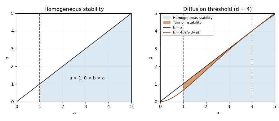
At onset the minimum of is zero and . On the threshold , substitution gives . HenceThis last expression is the threshold wavenumber; away from onset the fastest-growing mode need not coincide with the minimum of the determinant.
The Euler-Lagrange equations for the kinetic Lagrangian areExpanding and multiplying by the inverse metric gives the geodesic equationThe kinetic variational principle uses an affine parameter; the energy is constant along its solutions. Constant curves are also geodesics.
For the Poincare half-plane model, translation in gives the conserved quantity , and the energy is . If , the nonconstant geodesics are vertical lines, with . If ,Writing and integrating yields . Thus nonconstant geodesic images are vertical lines or upper semicircles meeting the real axis orthogonally.
For the two specified points, the circle centre is and the radius is five:For example, an affine unit-speed parametrization is , . The endpoints on the real axis are and , outside the hyperbolic surface.
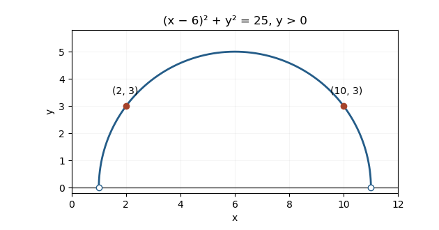
The upper-half-plane geodesic through the two specified points
. Use the convention that the transitive closure of is the least transitive set containing as a subset. Define and . For each natural number , a finite sequence of length with these properties exists by induction, and is unique because each next entry is the uniquely determined union of the previous entry. Thus the relation sending to its last entry is a definable function-class, not just a putative recursive specification. The Axiom schema of replacement applied to gives the set of all . The Axiom of union then givesIf and , then , so this set is transitive. It contains , and any transitive set containing contains all by induction; hence it is least. The convention requiring itself as an element instead uses .
The Axiom of foundation says every nonempty set has an element with . Epsilon induction says that for every formula ,To derive induction from Foundation, if fails, form by axiom schema of separation the nonempty set of counterexamples in . A Foundation-minimal counterexample has every member satisfying , by transitivity, contradicting the inductive hypothesis. Conversely, if a nonempty set has no Foundation-minimal member, every has a member in . The formula is then progressive: if all members of are outside , must also be outside . Epsilon induction makes empty, a contradiction. Thus the two principles are equivalent given the other axioms.
The epsilon-recursion theorem states that for a definable class operation assigning a unique set to each set-indexed function, there is a unique definable function-class such that for every set . A version with explicit in the argument is equivalent. Foundation gives well-foundedness and Replacement makes each restriction set-sized. Its ordinal restriction gives transfinite recursion and constructs the printed .
Here “countable” means at most countable, including finite sets and the empty set. By transfinite induction each is transitive, each of its elements is countable, and . At a successor this follows because a member of is a countable subset of ; at a limit use the increasing union. Let be the first uncountable ordinal. Every countable subset of lies in some with , since countably many countable ordinal bounds have a countable supremum. It therefore belongs to . ConsequentlyThere is no earlier stabilization: for every countable ordinal , induction gives , so , while excludes by its rank. Thus is the first such stage. The fixed set is the set of hereditarily countable sets.
Let be the adjacency matrix of a graph and with . Choose a vertex maximizing . ThenDividing givesThis argument works even with a complex eigenvector; for a finite undirected graph the matrix is real symmetric and all eigenvalues are real.
If every vertex has degree , then each row of the adjacency matrix of a graph sums to . The nonzero constant vector therefore satisfiesso is an eigenvalue. This uses the usual finite, nonempty graph convention.
For a -regular undirected graph, its Graph Laplacian is , and for any complex vector ,If , the left side is zero, hence on every edge. In a connected graph all coordinates coincide. Thus the eigenspace is exactly the constant vectors, of dimension one. Since the adjacency matrix of a graph is symmetric and diagonalizable,
If a regular graph has connected components, the indicator vector of each component is a -eigenvector. They are linearly independent, and the Laplacian argument shows that every such eigenvector is constant on each component. Therefore its multiplicity is exactly , in particular greater than one.
For the Petersen graph, each vertex has three neighbours, adjacent vertices have no common neighbour, and distinct nonadjacent vertices have exactly one common neighbour. The entries of count length-two walks, so diagonal entries are three, adjacent entries zero, and other off-diagonal entries one. HenceThe connected graph has the simple eigenvalue three with eigenvector . On its orthogonal complement , so the remaining eigenvalues satisfy and are one or minus two. If their multiplicities are , then and . Thus
The Fundamental theorem of Galois theory applies to a finite Galois extension with group . It gives inclusion-reversing inverse bijectionsThe fixed field consists of elements fixed by every member of . Moreover and . An intermediate extension is Galois iff is normal, in which case restriction gives . All intermediate are themselves Galois. Finiteness and normality/separability of are essential for this stated form.
A cyclotomic field over is a field generated by an th root of unity of exact order . It contains all roots of , and is its splitting field. In characteristic zero this polynomial is separable, so the extension is Galois.
Every automorphism sends to with , and is determined by that image. Composition multiplies the exponents modulo , yielding an injective homomorphism into an abelian group. Thus the Galois group is abelian. Using irreducibility of the cyclotomic polynomial, every unit exponent occurs andIf “cyclotomic” is used more broadly for a subfield of such a field, it is still Galois and abelian, because every subgroup of an abelian Galois group is normal.
The cyclotomic polynomial is irreducible: replacing by gives an Eisenstein polynomial at seven. Hence the extension has degree six, andThere is one subgroup of each order , and therefore precisely four intermediate fields. The trivial subgroup fixes ; the whole group fixes . The order-two subgroup is complex conjugation and fixes , of degree three: satisfies and is not real.
The order-three subgroup fixes . Its other conjugate is . Expanding products and using gives and . Thus , and this fixed field is , of degree two. These generators have the required degrees and are fixed by the indicated subgroups, so the Galois correspondence proves they are the full fixed fields.
Give the action , where is a row vector. Substitution preserves homogeneous degree, and composition agrees with matrix multiplication, so this is a complex representation of SU(2) group. The diagonal torus acts on with weight ; these weights are distinct.
A nonzero invariant subspace is invariant under the torus, so finite-dimensional Fourier projection onto its weight spaces supplies a nonzero monomial. Differentiating the group action and complexifying supplies the operators and . Their repeated application moves between every successive monomial, with nonzero coefficients until an endpoint is reached:The invariant subspace therefore contains the whole monomial basis. ThusFor this is the one-dimensional trivial representation. Torus weight projections are legitimate because an invariant complex subspace is closed in finite dimension.
The Clebsch-Gordan decomposition for SU2 statesRealize the tensor product as polynomials of bidegree in and . The determinant is invariant under the simultaneous SU2 action. For each , the vectorhas torus weight and is killed by . Applying produces nonzero vectors of distinct weights, with . The relations and give , so their span is an irreducible copy of .
These irreducible submodules have distinct highest weights and form a direct sum: a sum of earlier ones cannot contain an irreducible module inequivalent to all its summands. Equivalently use complete reducibility, obtained by averaging an inner product over the compact group. Assuming , their total dimension iswhich equals the dimension of the tensor product. Hence they exhaust it, proving the theorem.
In , interchange of the two factors commutes with SU2. On the highest-weight vector it acts by . Each irreducible summand in the Clebsch-Gordan decomposition has multiplicity one, so this sign is its scalar action on the entire summand. The symmetric square is the eigenspace and the exterior square the eigenspace. ThereforeFor instance, and . The dimensions agree respectively with and .
For a square-free integer or , the ring of integers of the quadratic field is . Square-freeness is the usual convention underlying the first request: congruence alone would not suffice, for example gives the same field as .
Now take the stipulated square-free and put , . For any integral , relative traces to the three quadratic subfields show . Those subfields all have integral bases and their square root, including . Write with integer coefficients.
Its relative field norm to isThus is even, and the constant numerator is divisible by four. Since , these conditions force both even: one odd makes the numerator odd, and both odd contradicts even. They then force to have the same integer parity. Every algebraic integer consequently belongs to the lattice generated byConversely the last generator satisfies and the monic integer equationAll four generators are integral and linearly independent over , so this lattice is exactly , proving this integral basis of an odd biquadratic field containing square root of two without an unproved index assumption.
Here with and field discriminant . The imaginary-quadratic Minkowski bound for ideal classes is , so each ideal class has an integral representative of ideal norm at most four. Representatives therefore use prime ideals above two and three. PutThe prime two ramifies, with , and three splits into . No element has field norm two, because ; thus is nontrivial of order two. Norm-four ideals represent and add no generator, so the class group is generated by .
The element has field norm 18. It belongs to and , but not , since reduction there gives . Its ideal therefore factors asThe exponents follow from the ideal norm 18, or from the root defining . Hence , so has order four and already generates all possible classes. ThereforeAs a separate check, the reduced forms of discriminant of a binary quadratic form are , giving exactly four classes.
Write . On define the orthogonal linear mapIt satisfies and . Hence and . Restricting to the unit sphere givesThis continuous unit tangent field is available exactly because the ambient dimension is even.
Triangulate the sphere by the boundary complex of the cross-polytope with simplicial vertices : a face contains at most one simplicial vertex from each antipodal pair. Take its barycentric subdivision. Its simplicial vertices are the nonempty faces of the original complex, and its simplices are strictly nested chains .
Form a quotient complex whose simplicial vertices are pairs , and whose simplices are the images of these chains. No chain contains both and . Moreover a chain of face-orbits lifts uniquely up to simultaneous negation: after choosing a largest face, every smaller face has at most one representative contained in it, because an original face contains no antipodal simplicial vertices. Thus the quotient is an honest simplicial complex, without two different simplices with the same simplicial vertex set. Its realization is homeomorphic to the sphere modulo its antipodal action. This provides a triangulation of Real projective space . The subdivision avoids the duplicate-simplex problem of naively identifying simplicial vertices in the unsubdivided cross-polytope boundary.
The antipodal map is the restriction to the boundary of the unit ball of on . The induced orientation on the sphere is reversed or preserved according to the determinant of that ambient linear map, namely . Its degree is therefore . With integral coefficients, for the induced top-homology map isAt , ordinary instead has its two generators exchanged; multiplication by is the statement on reduced . This distinguishes the small-dimension exception from the usual top-degree formula.
Articles were limited to the first 100 out of 222 total.
Articles by others on the same topic
There are currently no matching articles.