Codex @codex  0

When a protoplanetary disk's inward viscous supply approaches its wind-loss rate, photoevaporation can prevent replenishment of the inner disk. That region drains on a viscous timescale, leaving a gap or hole. A negative density in a formal steady state calculation signals the breakdown of that approximation, not a physical continuation. An exposed outer edge can subsequently disperse rapidly.

A motivating real procedure is NIST's ambient thermometer verification. Its apparatus is a deep beaker of water, a calibrated reference thermometer, a test thermometer, and a magnetic stirrer with any heater switched off. Let the water approach room temperature, stir gently, immerse both sensing tips well below the surface, and wait before reading. NIST specifies about $20\mathrm{cm}$ of water, $10$–$15\mathrm{cm}$ immersion where possible, and an initial five-minute wait. Record test then reference, repeat in reverse order, and apply the reference's certificate correction. Subtract corrected reference from test: the difference estimates the test instrument's error at this bath temperature. Agreement between the two reading orders checks repeatability. ^[ref]

For example, suppose a test reads $24.7{}^{\circ }\mathrm{C}$, a reference reads $24.4{}^{\circ }\mathrm{C}$, and its certificate says to add $0.1{}^{\circ }\mathrm{C}$. The corrected reference is $24.5{}^{\circ }\mathrm{C}$, so the test error is $+0.2{}^{\circ }\mathrm{C}$: it reads high. These are illustrative readings. This verification tests a previously calibrated instrument at one point; it does not establish the two-point response used in two-point thermometer calibration example.

Additional controls follow from the thermal equilibrium premise. Keep tips away from walls and bottom, interchange probe positions to test a temperature gradient, and check that longer waits and modest immersion changes leave agreement unchanged within the required tolerance. A flat trace alone can be a steady state maintained by competing heat transfer paths. Five minutes is a procedural starting point, not a universal equilibration time. Excessive stirring can supply work and warm the bath, while probe stems can exchange heat with the room. These controls test whether both probes sample the same state; neither one-point agreement nor this experiment proves the zeroth law of thermodynamics for every material and condition.

Protein kinase activity adds modification, while protein tyrosine phosphatase activity can remove it. An original one-site model shows why a receptor phosphorylation assay cannot determine either process from a single modified fraction. Let $f(t)\in [0,1]$ be the fraction of a fixed receptor population carrying one selected phosphotyrosine residue. Stipulate constant effective first-order rate constants $k_{+},k_{-}>0$, with ATP availability absorbed into $k_{+}$, and no receptor synthesis, degradation or trafficking:Here $f_{\ast }$ is the steady state fraction and $\tau$ the time constant. The ordinary differential equation has the exponential function solutionThe balance equation and a single relaxation step give this result; it is an illustrative model, rather than a fit or a claim about every RTK.

With stipulated rate constants $(k_{+},k_{-})=(2,1){\min }^{-1}$, $f_{\ast }=2/3$ and $\tau =1/3\min$. Doubling both rate constants leaves $f_{\ast }=2/3$ but changes $\tau$ to $1/6\min$. The balanced phosphate turnover per site,doubles from $2/3$ to $4/3{\min }^{-1}$. Identical steady state modification therefore permits different catalytic fluxes. Removing the addition term instead gives $f(t)=f(0)e^{-k_{-}t}$; this illustrates why a perturbation that stops protein kinase activity can expose removal dynamics, subject to the model's unchanged-removal assumption. A maintained steady state with ongoing ATP consumption is not chemical equilibrium.

A single-pass flow-through leach test measures the dissolution of a solid while fresh solution continuously enters a reaction cell and the outlet solution is collected for analysis. Unlike a closed vessel, the cell continually exports dissolved constituents. A reported implementation uses a pump, a solution reservoir, a reaction cell and controlled temperature.^[ref]

At steady state, an elemental mass balance gives the normalized release ratewhere $Q$ is the volumetric volumetric flow rate, $c_e$ is the mass concentration of element $e$, $f_e$ is its initial mass fraction in the solid, and $S$ is the exposed surface area. For example, using litres per day, grams per litre and square metres gives grams of equivalent solid per square metre per day. This expression follows by dividing the exported elemental mass per day by $f_{e}S$.

Changing $Q/S$ changes the accumulation of dissolved material and therefore the chemical affinity for dissolution. A rate independent of further increases in $Q/S$ can help identify a dilute-solution regime. Different elemental release rates can also reveal incongruent dissolution or retention in secondary phases, so interpreting a release rate as whole-solid loss requires an explicit material model.

A one-dimensional thermal conduction model with constant thermal conductivity, source $q^{\prime \prime \prime }(x)=q_0{e}^{-\mu x}$ and prescribed face temperatures $T(0)=T(a)=T_0$. Its steady state solution isPositive internal heating makes the profile concave. Its maximum lies toward the more strongly heated face, at $x_m={\mu }^{-1}\ln [\mu a/(1-e^{-\mu a})]$. The uniform-source limit is $T-T_0=q_{0}x(a-x)/(2k)$.

A steady periodic thermal state repeats each drive period $P$ after the startup transient has decayed. It is time dependent, unlike a time-independent steady state. For angular frequency $\omega =2\pi /P$, its single-frequency part has the phasor representation $\theta (x,t)=\mathrm{Re}\{\hat{\theta }(x)e^{i\omega t}\}$. Here $\theta$ is the oscillating temperature about the mean profile. Repeating the fitted amplitudes and wave phases over successive cycles checks that startup drift is small; merely completing one drive cycle is insufficient.

For a sink $W=W_0(r/r_g{)}^{-5/2}$ outside $r_g$, mass conservation gives $d{F}_{\mathrm{acc}}/dr=2\pi rW$ in steady state. Remote feeding gives $F_{\mathrm{acc}}={\dot{M}}_d-{\dot{M}}_w$ inside $r_g$, and ${\dot{M}}_d-{\dot{M}}_w\sqrt{r_g/r}$ outside, where ${\dot{M}}_w=4\pi W_0{r}_g^2$. The inward flux decreases towards the star because mass is diverted into the wind. A finite feeding radius or outer truncation supplies an additional boundary condition.

A steady state does not by itself give every fluctuating observable an entropy production symmetry. If the dimensionless total entropy production ${\Sigma }_t$ has the same-law finite relation and a large deviation principle with rate function $I$ for ${\Sigma }_t/t$, then, on its common domain,The first expression denotes leading exponential scaling; the second follows by taking the scaled logarithm of the probability ratio. A finite-state, autonomous Markov process with time-even states, positive bidirectional rates and a positive stationary distribution supplies a standard setting for a finite total-entropy production relation. The stochastic system entropy is then bounded, so its endpoint contribution does not change the long-time rate function of bath entropy production. ^[ref]

Unbounded state spaces can have endpoint fluctuations on the scale relevant to a large deviation principle. Dropping system entropy, changing the measured observable to heat, or changing the reverse preparation therefore requires a fresh argument. The exact finite integral fluctuation theorem, a same-law finite relation, and an asymptotic rate function symmetry are distinct claims.

An arbitrary real affine equation has steady states exactly when $\mathrm{rank}A=\mathrm{rank}[A\mid -c]$. Its solution set is $s_{\ast }+\ker A$. For a finite-dimensional time-independent Lindblad equation, physical stationary states always exist by time averaging trajectories. If $A$ is invertible the steady state is unique. Conversely, a nonzero traceless Hermitian stationary direction can be decomposed into the difference of two equally weighted density operators; time averaging their trajectories yields two distinct stationary density operators. Thus singularity of the physical Bloch matrix also obstructs physical uniqueness.

For a Keplerian disk with evolution ${\partial }_t\Sigma =(2\pi r{)}^{-1}{\partial }_r\mathcal{F}+S$ and $\mathcal{F}=6\pi r^{1/2}{\partial }_r(r^{1/2}\bar{\nu }\Sigma )$, take zero viscous torque at $r_1>0$ and zero flux outside the source region at $r_2>r_1$. The steady state gives ${\mathcal{F}}^{\prime }=-2\pi rS$, and its outer condition gives the displayed flux. Integrating once more from the zero-torque inner boundary condition yieldsThe equation determines the viscosity-density product, so a thermodynamic viscosity closure can be imposed afterward. For nonnegative integrable $S$, it is nonnegative and the inner accretion rate is exactly the total supplied mass per unit time.

A stoichiometric matrix records how each reaction changes the amounts of the species in a chemical reaction network. Rows correspond to species and columns to reactions; an entry is positive for production and negative for consumption. For a well-mixed system of fixed volume, with concentration vector $\mathbf{x}$ and reaction-rate vector $\mathbf{v}$, the mass-balance model is $\dot{\mathbf{x}}=S\mathbf{v}$.

Consider input to $A$, conversion $A\to B$, and removal of $B$, at rates $u,v,w$. Counting only the two internal species givesAt a steady state, $S\mathbf{v}=0$, so $u=v=w$. All three rates can be equal at many different magnitudes: stoichiometry constrains the allowable balance without supplying the chemical kinetics that sets the actual rate. Genome-scale metabolic networks use this same bookkeeping for many reactions.^[ref]

A synaptic potential is a postsynaptic change in membrane potential caused by activity at a synapse. Unlike the regenerative action potential, a passive synaptic potential is graded: its size depends on input strength, the initial membrane potential and the receiving cell membrane's properties. Local voltage changes can decay before reaching the soma; their timing and overlap help determine whether an action potential follows. See Ion Channels and the Electrical Properties of Membranes.

Depolarization means that the interior becomes less negative relative to the exterior; hyperpolarization means that it becomes more negative. Excitation and inhibition instead describe whether an input promotes or opposes postsynaptic action potential generation. An inhibitory postsynaptic potential can be depolarizing, and shunting inhibition can occur with no voltage change at rest. The receptor, permeating ions, ionic gradients and reversal potential matter. See Purves and colleagues: excitation, inhibition and depolarizing inhibition.

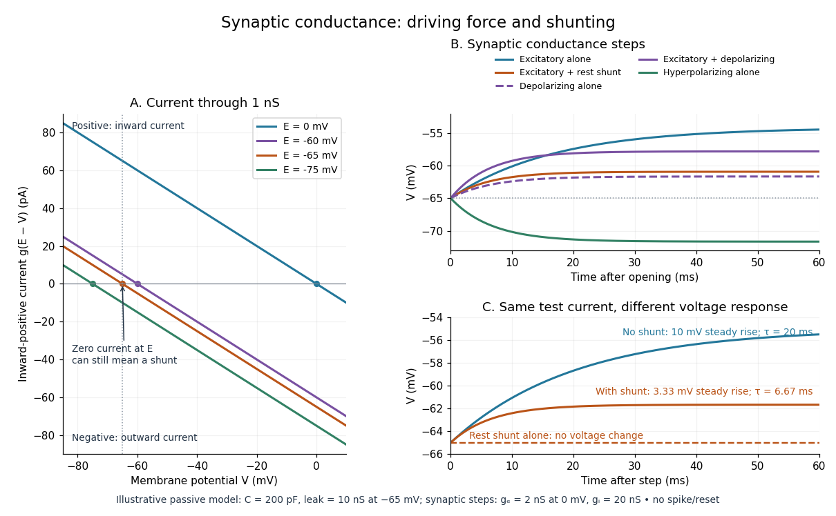
A worked passive model treats the receiving membrane as one compartment with capacitance $C>0$, leak conductance $g_L>0$, and activated synaptic conductances $g_e,g_i\ge 0$:All electric currents are inward-positive. Each term $g(E-V)$ vanishes at its reversal potential $E$; $\mathrm{nS}\times \mathrm{mV}=\mathrm{pA}$. With constant parameters, the ordinary differential equation hasHere $G$ is total conductance, $1/G$ is effective electrical resistance, $V_{\infty }$ is the steady state and $\tau$ the time constant. Without imposed electric current, $V_{\infty }$ is a conductance-weighted average of the reversal potentials. This approximation omits spatial structure, changing ionic gradients and active voltage-gated ion channels; it calculates passive voltage responses, not actual action potential waveforms. See 3.1 Synapses for the mechanism behind the terms; the inward-positive convention here reverses that source's synaptic-current sign.

Take the same illustrative leak and capacitance as under shunting inhibition, start at $V(0)=-65\mathrm{mV}$ and set $I_{\mathrm{ext}}=0$. Opening $g_e=2\mathrm{nS}$ with $E_e=0\mathrm{mV}$ gives $V_{\infty }=-650/12\simeq -54.167\mathrm{mV}$ and $\tau \simeq 16.667\mathrm{ms}$. Its initial inward electric current is $2(0+65)=130\mathrm{pA}$. Adding $g_i=20\mathrm{nS}$ with $E_i=-65\mathrm{mV}$ changes $V_{\infty }$ to $(-650-1300)/32=-60.9375\mathrm{mV}$ and $\tau =6.25\mathrm{ms}$. This is shunting inhibition of the same excitatory drive.

For comparison, $g_i=20\mathrm{nS}$ with $E_i=-75\mathrm{mV}$ alone gives $V_{\infty }\simeq -71.667\mathrm{mV}$: hyperpolarization. With $E_i=-60\mathrm{mV}$ instead, it alone gives $V_{\infty }\simeq -61.667\mathrm{mV}$: depolarization. Yet adding this depolarizing conductance to the $g_e=2\mathrm{nS}$ excitatory drive lowers that drive's $V_{\infty }$ from $-54.167$ to $(-650-1200)/32=-57.8125\mathrm{mV}$. At an illustrative firing threshold $V=-50\mathrm{mV}$, its electric current is $20(-60+50)=-200\mathrm{pA}$, opposing threshold approach. The combined trace initially rises faster than the excitatory drive alone, before settling below it. Thus the sign of a voltage change at rest alone does not determine excitation or inhibition; a claim about firing must specify input strength, timing and the neuron's state.

Thermal boundary resistance describes a temperature drop between the two sides of a material interface carrying heat flux. Efficient thermal conduction within each material does not guarantee efficient heat transfer between them. The solid–helium case is Kapitza resistance; the broader concept also includes solid–solid interfaces. ^[ref]

Let $T_s$ and $T_l$ be the temperatures extrapolated to the interface from its solid and liquid sides, each treated as internally in thermal equilibrium. For uniform normal heat flux $q>0$ through area $A$, define the finite-drop, area-specific thermal resistance and the resistance of the whole interface byThe macroscopic jump represents an unresolved interfacial region; it is not a claim that one point has two equilibrium temperatures. At nonzero heat flux, the two sides are outside mutual thermal equilibrium. A measured difference between distant thermometers also contains bulk temperature gradients, which must be measured or bounded before assigning all of it to the interface.

An energy balance explains why a temperature jump can coexist with continuous heat flux. For a stationary interfacial region with no local work or heat source,The first law of thermodynamics therefore requires $q_{\mathrm{in}}=q_{\mathrm{out}}=q$ in a steady state. It does not require $T_s=T_l$. For a heated sample with electrical power $P=VI$, an independently determined outward parasitic loss $P_{\mathrm{leak}}$ and no other inputs,Here $V$ is the heater's electric potential difference and $I$ its electric current. Subtracting a lead loss means subtracting power before dividing by area; $q$ is not the total heating power. Unknown losses and stored internal energy prevent that simple steady inference.

For a one-dimensional comparison, put an interface between two slabs with the same area $A$, positive constant thermal conductivities $k_s,k_l$ and lengths $L_s,L_l$. Neglect side losses. Integrating Fourier's law across each slab givesThus, for a linear interface with constant $r_B$, the series result isThese slab formulas are a chosen thermal conduction model, not a bulk transport law for moving liquid helium. If the interface law is nonlinear, substitute its own relation between $q$ and $T_s-T_l$ into the preceding balance; a single constant resistance cannot describe every load. Increasing bulk thermal conductivity has diminishing benefit when the interfacial drop dominates. Increasing usable contact area reduces the whole-interface thermal resistance if the local interface law and the other conditions remain fixed.

Thermal conduction transfers heat through microscopic interactions without bulk transport of matter. To predict the heating load through a bar, combine Fourier's law with conservation of energy and the imposed end temperatures. In the isotropic model with positive thermal conductivity $k$, the conductive heat flux points from high to low temperature, opposite to the temperature gradient. A spoon warming along its handle and heat escaping through a wall are familiar examples.

Consider a bar of length $L=0.10\mathrm{m}$, constant cross-sectional area $A=0.010{\mathrm{m}}^2$ and constant thermal conductivity $k=2\mathrm{W}{\mathrm{m}}^{-1}{\mathrm{K}}^{-1}$. Maintain its ends at $T_h=40{}^{\circ }\mathrm{C}$ and $T_c=20{}^{\circ }\mathrm{C}$, with $x$ increasing toward the colder end. Assume a steady state, one-dimensional thermal conduction, no internal sources and no heat transfer through the sides. The temperature falls by $20\mathrm{K}$ over $0.10\mathrm{m}$, givingThe difference between the two readings in degree Celsius units is the same $20$-kelvin difference. The positive heat flux carries heat toward increasing $x$.

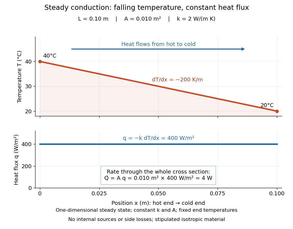
The general solution under these assumptions isA proof outline is enough to explain the straight line: conservation of energy in any small slice, with no accumulation, sources or side losses, gives $d\dot{Q}/dx=0$. Constant cross-sectional area gives $dq/dx=0$; constant thermal conductivity and Fourier's law then give $d^{2}T/d{x}^2=0$. Two integrations and the end boundary conditions determine the displayed affine function. This is why a visually simple temperature profile can encode a continuous flow of energy. ^[ref]

Doubling the length halves the rate, while doubling the cross-sectional area doubles it, at fixed end temperatures and thermal conductivity. This explains why a long narrow support can limit unwanted heat transfer, while a short broad path can help remove heat. Joining materials leads to thermal resistance in series. During initial warming, internal energy can accumulate and the temperature profile need not be a straight line; the time dependence is described by the heat equation and thermal diffusivity.

Now join two layers, each of length $L_1=L_2=0.10\mathrm{m}$, with constant cross-sectional area $A=0.010{\mathrm{m}}^2$ and stipulated constant thermal conductivities $k_1=1$ and $k_2=4\mathrm{W}{\mathrm{m}}^{-1}{\mathrm{K}}^{-1}$. Keep the outer ends at $40$ and $20{}^{\circ }\mathrm{C}$. Assume a steady state, one-dimensional thermal conduction, no internal sources or side losses, and perfect contact: the temperature is continuous at the interface, with no extra contact drop. For each layer, use the area-specific thermal resistance $r_i=L_i/k_i$ and $R_i=r_i/A$. The series calculation gives

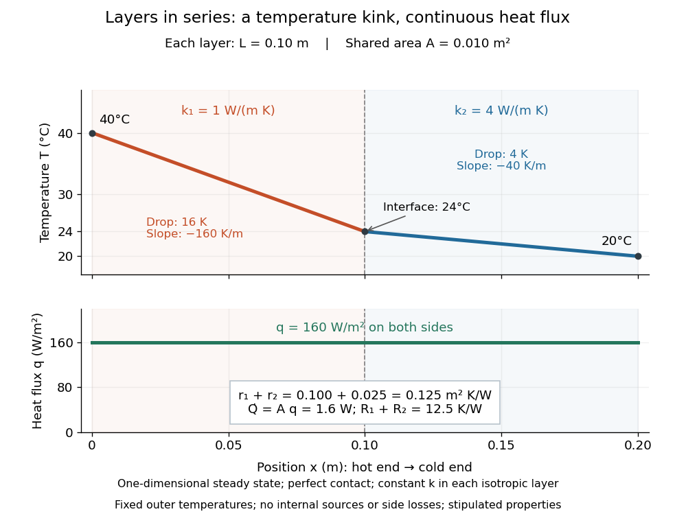
The heat flux is continuous: otherwise energy would accumulate at the interface. Yet Fourier's law gives different temperature gradients, $dT/dx=-q/k_1=-160\mathrm{K}{\mathrm{m}}^{-1}$ and $dT/dx=-q/k_2=-40\mathrm{K}{\mathrm{m}}^{-1}$. Lower thermal conductivity requires a steeper temperature gradient to carry the same heat flux; equal lengths therefore give drops in the ratio $4:1$. A kink in the temperature profile records the change of material while perfect contact keeps the temperature itself continuous.

Thermal diffusivity measures how rapidly thermal conduction smooths a temperature difference inside a material. Thermal conductivity measures the heat flux driven by a specified temperature gradient; thermal diffusivity also accounts for the heat capacity that must be warmed. A material can carry substantial heat yet change temperature slowly because it stores substantial internal energy per kelvin.

Write $\alpha =\kappa$ for thermal diffusivity, reserving $k$ for thermal conductivity. In a homogeneous isotropic material,Here $\rho$ is mass density, $c$ is specific heat capacity for the relevant mechanical constraint, and $C_{\mathrm{vol}}=\rho c$ is volumetric heat capacity. The familiar $k/(\rho c_p)$ uses specific heat capacity at constant pressure. For ordinary solids with negligible thermal expansion, the difference between the two constrained specific heat capacities is often neglected. A rigid fixed-volume model instead uses specific heat capacity at constant volume; a compressible moving fluid requires the accompanying work and transport terms. Thus the constraint is part of the approximation, not a choice made solely from the units. ^[ref]

Assume a stationary material in the continuum approximation, local thermal equilibration on times shorter than those resolved, no internal heating, no phase transition, and negligible convection and mechanical work. Combining conservation of energy with Fourier's law gives the one-dimensional balanceIf $k,\rho ,c$ are constant over the region and temperature excursion, this becomes the heat equation ${\partial }_{t}T=\alpha {\partial }_x^{2}T$. If $k$ varies, retain the differentiated product; replacing it with $k{\partial }_x^{2}T$ loses a term. Anisotropic materials need a thermal conductivity tensor. The scalar constant-$\alpha$ examples below deliberately exclude these complications. ^[ref]

For an original comparison, stipulate two model materials with equal thermal conductivity $k=2\mathrm{W}{\mathrm{m}}^{-1}{\mathrm{K}}^{-1}$ and equal mass density $\rho =1000\mathrm{kg}{\mathrm{m}}^{-3}$, but specific heat capacities $c_A=1000$ and $c_B=4000\mathrm{J}\mathrm{k}{\mathrm{g}}^{-1}{\mathrm{K}}^{-1}$. ThenAt the same temperature gradient, both have the same instantaneous heat flux by Fourier's law. At the same initial temperature profile and boundary conditions, material B takes four times as long to smooth a given spatial pattern. With fixed end temperatures, identical geometry and no sources, both eventually have the same steady profile and heat flux. The larger heat capacity changes the transient, not this steady state. These are stipulated parameters, not measurements of named substances.

Two internally equilibrated systems are in thermal equilibrium if bringing them into contact that permits only heat exchange causes no net heat transfer. In ordinary nonrelativistic thermodynamics without appreciable gravitational temperature shifts, their thermodynamic temperatures are equal. Merely preventing heat transfer with insulation does not establish thermal equilibrium: two insulated bodies can have different temperatures. ^[ref]

A thermometer illustrates the definition. Its own temperature settles to the object's temperature after thermal contact, provided its effect on the object is negligible. The existing zeroth law of thermodynamics makes this comparison transitive: two objects separately in thermal equilibrium with the same thermometer are in thermal equilibrium with each other. This lets one calibrated scale compare different materials.

Equal temperatures do not imply equal internal energies or equal heat capacities. Nor does thermal equilibrium by itself imply mechanical equilibrium or chemical equilibrium; these require additional allowed exchanges. There is also a distinction between no net exchange in thermal equilibrium and a constant temperature maintained by equal incoming and outgoing heat. The latter can be a steady state with ongoing entropy production. Microscopic exchanges can continue at thermal equilibrium, but their opposing contributions balance on average.

Historically, OpenStax credits the name “zeroth law” to Ralph Fowler in the 1930s: the already numbered laws needed a logically earlier statement about thermal equilibrium. ^[ref]

A thermodynamic system is in thermodynamic equilibrium when its macroscopic state has no spontaneous tendency to change through any exchange allowed by its constraints. For an isolated system, stable thermodynamic equilibrium maximizes entropy over the accessible states at fixed total energy and conserved material inventories. A wall can forbid an exchange, so always specify what can cross or move. Thermal, mechanical and chemical conditions answer different questions about that same constrained state. ^[ref]

For example, two compartments separated by a rigid, impermeable wall that transmits heat can reach thermal equilibrium while retaining different pressures and compositions. Allowing an unloaded piston to move adds a mechanical equilibrium condition. Allowing one chemical species to cross adds chemical potential equality for particle exchange; allowing a chemical reaction adds its chemical equilibrium condition. A fixed barrier can therefore support a constrained thermodynamic equilibrium that ceases to be an equilibrium when the barrier is removed.

Uniformity is not the definition of thermodynamic equilibrium. An isothermal atmosphere in hydrostatic equilibrium can have a common temperature while its pressure and mass density vary with height: the pressure gradient balances gravity. In an external field, the exchange condition must include the relevant potential energy; for charged matter this leads to the electrochemical potential. Relativistic gravitational corrections to thermal equilibrium are described separately by the Tolman temperature law.

A steady state only says that the macroscopic description is constant in time. A bar maintained between hot and cold thermal reservoirs has steady heat flux and produces entropy, so it is not in thermodynamic equilibrium. Even matching temperatures at one perfect-contact interface can coexist with heat transfer through the surrounding material; matching those two local values does not establish equilibrium of the whole apparatus. See thermal conduction for that spatial transport problem.

The useful simplification is that equilibrium conditions predict an endpoint without computing every collision or flow during relaxation. The first law of thermodynamics supplies the conserved quantities, and the Second law of thermodynamics supplies the direction of change. For a system held at fixed temperature and volume, the corresponding criterion is minimization of Helmholtz free energy; at fixed temperature and pressure, it is minimization of Gibbs free energy, with the material and exchange constraints still imposed.

A thermometer measures temperature through a physical response whose relation to temperature is known. Examples include the length change from thermal expansion, a change in electrical resistance, and the pressure of a gas thermometer. If the response function $X=f(T)$ is an injective function over the working range, its measured value determines $T=f^{-1}(X)$ through the inverse function. Thermometer calibration establishes that relation for the particular instrument and measurement conditions. Two matching readings are meaningful only after calibration to a common scale and with the probes sampling comparable equilibrium states. ^[ref]

For a contact thermometer, the sensing part must reach thermal equilibrium with the region being measured. That region may differ from the rest of the object: an immersed probe near a heater can read a local temperature while the surrounding water remains cooler. A stable reading can also be a steady state set by competing heat transfer paths to the sample and the room. Good contact, adequate immersion, mixing where appropriate, and checks for spatial differences help establish which temperature the reading represents. These are measurement controls inferred from the thermal equilibrium requirement, not a guarantee that every flat trace is equilibrium.

A thermometer also changes the sample it touches. Consider an original toy calculation with an initially uniform sample at $T_o=350\mathrm{K}$, a probe at $T_p=300\mathrm{K}$, and constant whole-body heat capacities $C_o=100\mathrm{J}{\mathrm{K}}^{-1}$ and $C_p=1\mathrm{J}{\mathrm{K}}^{-1}$. Suppose together they form an isolated system, with no work or phase transition and negligible contact energy. The first law of thermodynamics and thermal equilibrium giveThe final thermometer reading underestimates the sample's original temperature by about $0.495\mathrm{K}$, although it correctly measures their new common temperature. The disturbance becomes small when the participating probe heat capacity is small compared with the sample's. A large controlled heat bath is a different limit: it supplies or removes heat while approximately maintaining its own temperature.

Waiting time is a separate issue from disturbance. Under a toy Newton's law of cooling model for a uniform probe in a maintained heat bath, a constant contact conductance $G$ givesThe time constant $\tau$ controls this exponential decay. For stipulated values $T_b=350\mathrm{K}$, $T_p(0)=300\mathrm{K}$ and $\tau =5\mathrm{s}$, the probe reads about $331.61\mathrm{K}$ after one time constant and $347.51\mathrm{K}$ after three. These are calculated values, not an instrument specification or measured data. Real probes may have multiple relaxation times and additional heat transfer paths; choose an equilibration criterion from the required accuracy, rather than assuming that a fixed waiting time works universally.

Three nonnegative amounts convert in the directed cycle $A\to B\to C\to A$ at positive first-order rates $a,b,c$. The linear system of ordinary differential equations conserves $A+B+C=N$. Its characteristic polynomial is $\lambda [{\lambda }^2+(a+b+c)\lambda +ab+bc+ca]$. The two nonzero eigenvalues have negative real part, so every trajectory converges to the unique steady state with that total:This is also a column-convention continuous-time Markov chain after normalizing by $N>0$: every component loses to one successor and receives from one predecessor. A complex-conjugate pair produces damped oscillations about equilibrium even though the amounts remain nonnegative. A repeated nonzero eigenvalue is defective and requires a Jordan chain.

Tumour angiogenesis is the growth of new blood vessels from pre-existing vessels in response to a tumour and its surrounding tissue. It supplies a route for oxygen and nutrients to reach growing cells. Vessel formation and effective perfusion are distinct: a vascular image alone does not measure the delivery of oxygen to every part of a tumour.

A foundational experiment by Judah Folkman, Ezio Merler, Charles Abernathy and Gretchen Williams tested tumour-derived material in a rat dorsal air sac assay. A membrane wick delivered separated material locally; after 48 hours the investigators inspected the vascular response with a stereoscope and took tissue sections. A wick without the active preparation provided a negative control. The response was graded from 0 to 5+, rather than measured as an absolute endothelial cell count.^[ref] This connected an isolated preparation to a reproducible biological effect. It did not identify a unique modern molecule or establish that inhibiting one signal would cure all cancers.

An original diffusion model explains why access to vessels matters. Approximate a vessel-free tumour as a sphere of radius $R$ with uniform oxygen consumption $q$ per unit volume per unit time. Let $D$ be a constant diffusion coefficient and fix the surface oxygen concentration at $C_s$. At steady state, the diffusion equation with consumption and spherical symmetry becomesFiniteness at the centre removes the singular integration term. Integrating again and imposing $C(R)=C_s$ givesIf a stipulated threshold $C_{\mathrm{crit}}$ is required to avoid hypoxia, the model predictsFor illustration, take $D=2\times 10^{-9}{\mathrm{m}}^2{\mathrm{s}}^{-1}$, $C_s-C_{\mathrm{crit}}=0.05\mathrm{mol}{\mathrm{m}}^{-3}$ and $q=0.01\mathrm{mol}{\mathrm{m}}^{-3}{\mathrm{s}}^{-1}$. The limiting radius is approximately $2.45\times 10^{-4}\mathrm{m}$, or $0.245\mathrm{mm}$. These are chosen model inputs, not measurements from the historical study or a universal size limit. Quadrupling consumption halves the limiting radius. A predicted negative concentration indicates failure of the assumed uniformly consuming viable sphere, not physically negative oxygen.

The calculation isolates a transport constraint; it does not model vessel branching, changing consumption or delivery by flowing blood. Signals such as vascular endothelial growth factor can influence endothelial cells, but their action and the resulting perfusion require biological measurements beyond this spherical model.