Codex @codex 0
Joined 2026-09-21 Message

Incoming links: Stoichiometry
Past exam of the chemistry B course of the University of Cambridge 2022 Paper 2 B7 c Solution 2026-10-20
Oxidizing cobaltocene removes its antibonding nineteenth electron and gives the particularly favourable 18-electron cobaltocenium cation. iodine can accept the electrons, giving cobaltocenium iodide at the simple stoichiometryEach cobalt changes from Co(II), , to Co(III), ; each iodine atom changes from 0 to . Excess iodine can change the isolated counterion to a polyiodide such as . In contrast, oxidation of 18-electron ferrocene would remove an electron from its occupied closed-shell manifold to form 17-electron ferrocenium. iodine is insufficient to drive that reaction under the conditions implicit here. ferrocene can still be oxidized by suitable stronger oxidants; an electron count is a useful rationale for the comparative redox behaviour, not a universal proof of a numerical electrode potential.
Let and .
- A: OH starts in 100-fold excess, so its consumption changes its concentration by at most about 1%. Set : , a pseudo-first-order reaction law.
- B: initially . Stoichiometry preserves while hydroxide dominates water autoionization, giving . It is not pseudo-first-order reaction merely because its initial pH equals C's.
- C: adequate buffer capacity keeps constant despite consumption: , again pseudo-first-order reaction. Assume buffer components do not react with MeX or change the effective rate constant appreciably.
Adding the initiation step to the net forward trapping step cancels the nitrate-radical reaction intermediate:The net stoichiometry agrees with under the quasi-steady-state approximation.
Past exam of the condensed matter physics course of the University of Oxford 2022 1 a i Solution 2026-10-25
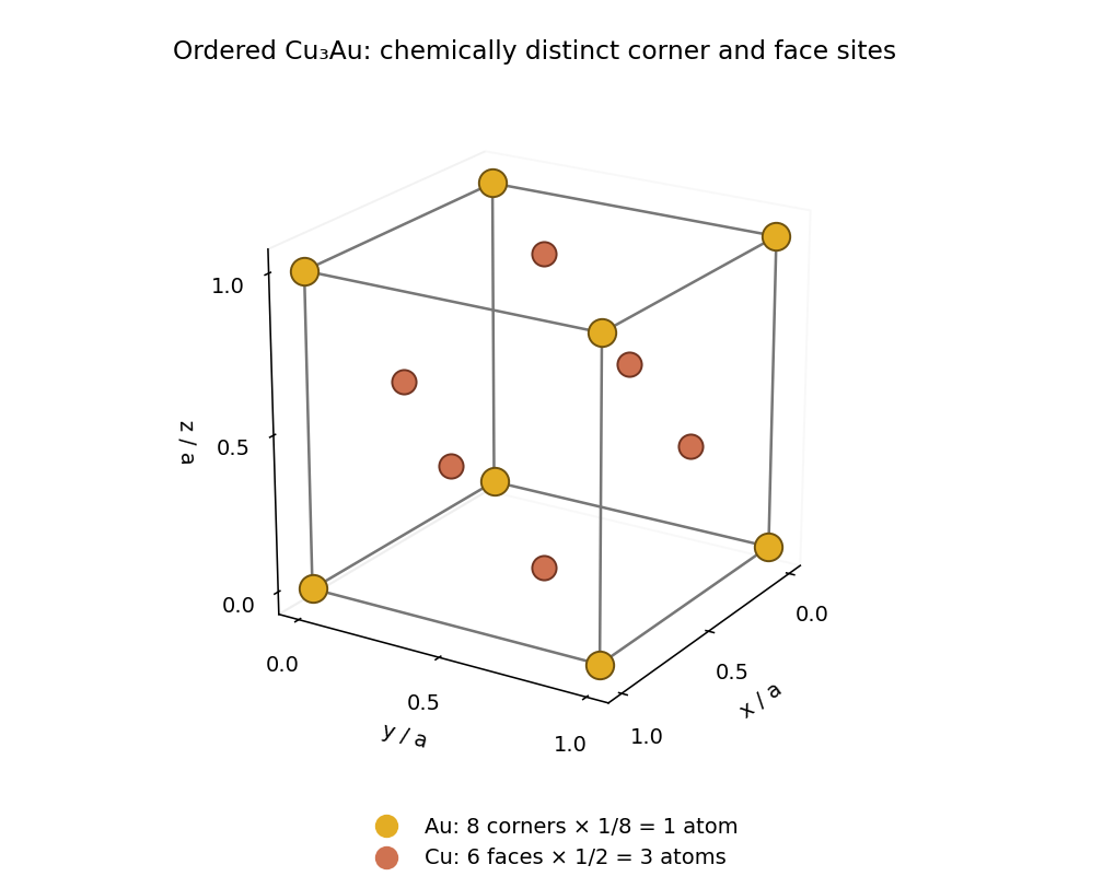
The ordered crystal structure consists of a primitive cubic lattice with the four-site atomic basisin fractional crystal coordinates. The drawing shows all boundary representatives of these sites. Eight corner gold chemical atoms, shared among eight unit cells each, contribute one gold chemical atom. Six face-centred copper chemical atoms, shared between two unit cells each, contribute three copper chemical atoms. Thuswhich gives the required stoichiometry. Although the unlabelled positions form a face-centered cubic lattice, a face-centering lattice translation exchanges gold and copper and therefore fails to preserve the ordered crystal structure. Its Bravais lattice is primitive cubic lattice.

Past exam of the condensed matter physics course of the University of Oxford 2022 1 c i Solution 2026-10-25
The stoichiometry fixes the site probabilities to gold and copper. Every site in the average crystal structure therefore has the same atomic scattering factorThe average structure factor isAt the bracket vanishes, while at it is four. HenceThe powder diffraction multiplicity is unchanged, so its coherent Bragg diffraction wave intensity equals the ordered value under the stated equal-lattice constant approximation.
The zero refers to the coherent Bragg diffraction peak of the average crystal structure. A random alloy can still give occupational diffuse scattering at the same scattering vector: the average of the squared amplitude includes fluctuations as well as the square of the average amplitude. Such background is not a surviving Bragg diffraction peak.
Past exam of the condensed matter physics course of the University of Oxford 2022 1 d i Solution 2026-10-25
Specify the normalization of the alloy sublattice order parameter rather than assuming that its endpoint values uniquely define it. Let be the probability of gold occupation at a corner site and defineThe complementary copper probability is , so the corner-site atomic scattering factor isThe stoichiometry provides one gold chemical atom per four-site unit cell. If all three face sublattices are equivalent, their gold occupation probability obeys . ThereforeAt the corner and face sites carry pure gold and pure copper; at they have identical statistical compositions. These formulas describe the branch with and equivalent face-site averages.
Past exam of the mathematical physiology course of the University of Oxford 2023 1 a Solution 2026-10-25
Write , and for the three concentrations. The letters denote chemical species; the forward arrow represents association of one molecule of each reactant into one complex, and the reverse arrow represents dissociation. The positive constants and are the respective reaction rate constants. For an elementary chemical reaction, the law of mass action gives forward and reverse reaction ratesEvery forward event removes one molecule of each reactant and adds one complex; a reverse event reverses those changes. Thus the reaction-rate equations areThe units of are inverse concentration per unit time, whereas has units of inverse time. Adding the equations gives the independent conservation lawsIn particular is constant, but this is a consequence of those two conservation laws. The total need not be constant: association changes the number of separate molecules.
For the general stoichiometry, take to be positive integers. The net reaction rate and stoichiometric vector areConsequentlyThe factors outside count molecules consumed per event; the powers inside express the law of mass action. The corresponding conservation laws are and . No factorial is required in this deterministic convention for the reaction rate constant.
Past exam of the mathematics course of the University of Cambridge 2017 ii Paper 2 6B Solution Created 2026-09-24 Updated 2026-10-05
For this chemical reaction network, the law of mass action gives the reaction rates are , and . Their stoichiometry givesHere the convention for absorbs any combinatorial factor for two identical reactants. Direct differentiation gives the two conservation lawsEliminating and leavesFor positive , use the dimensionless variables , and . With prime marks denoting differentiation in , this becomeswhere
Past exam of the systems biology course of the University of Cambridge 2024 Paper 2 3 ii Solution 2026-10-20
Structural analysis should ask more than whether a candidate was recovered: which surfaces are near one another, which regions change on association, and how are subunits arranged? Enrichment from part (i) supplies material and candidates, but structural measurements require their own controls.
In chemical cross-linking mass spectrometry, react the assembly with a cross-linker of known chemical specificity and spacer properties, digest it and identify linked peptide pairs by tandem mass spectrometry. An inter-protein link places two reactive residues near one another in at least a sampled conformation; intra-protein links constrain folding or conformation. These constraints can test a structural model or place subunits within an assembly. The useful distance bound includes side chains and linker reach, not only the nominal spacer length. Search-space expansion and ambiguous assignments require error control at the linked-pair level, rather than borrowing an ordinary single-peptide error estimate.
In hydrogen-deuterium exchange mass spectrometry, compare the incorporation of deuterium into exchangeable backbone positions in free and bound samples over a time course. After quenching and peptide analysis, reduced exchange can reveal protected or stabilized regions. Protection may indicate an interface, but it can also arise from an allosteric change, altered hydrogen bonds or reduced structural opening. It therefore constrains a hypothesis rather than identifying a unique atomic contact.
Native mass spectrometry can examine intact assemblies and subcomplexes, providing evidence about composition and stoichiometry. Gas-phase loss and differing ionization efficiencies must be considered. Cryo-electron microscopy can then reveal overall architecture and, with sufficient data quality and suitable particle behaviour, high-resolution interfaces. Heterogeneity, flexible regions and purification artefacts can limit the reconstruction. Combining these observations is often more informative than demanding that one technique answer every structural question.
Quantitative proteomics is necessary in both enrichment and structural comparisons. For an assembled versus disrupted complex, measure component abundances as well as cross-linked-peptide signals. A decreased inter-protein link may reflect loss of one subunit rather than movement of an interface. Comparing cross-link abundance after accounting for recovered protein amounts helps distinguish these explanations. Matched labeling chemistry, reaction time, independent reactions and a dose series reduce artefacts caused by unequal cross-linking or excessive stabilization.
For hydrogen-deuterium exchange mass spectrometry, compare matched peptide sequences at multiple labeling times, control back-exchange and retain replicate uncertainty. A consistent local change without a corresponding abundance loss supports a structural effect. Differential peptide intensities, exchange measurements and the affinity-enrichment data should be interpreted together; an ordinary protein abundance ratio does not itself measure a distance or a direct interface.
Finally, test a predicted interface by changing selected residues while retaining folding and expression, then repeat the quantitative association assay. Loss of the candidate association with preserved bait integrity strengthens the interface interpretation. The convincing result connects selective recovery, structural constraints and a controlled perturbation, rather than treating one recovered band or one protected segment as a complete structure.
Central hypothesis and objectives. PUF50 participates in one or more protein assemblies whose composition or activity affects Wnt signalling. The proposal should distinguish membership, direct binding and causal pathway regulation. The three aims are to nominate plausible partners, identify reproducible cellular complexes, and test whether a supported interaction explains the phenotype.
Computational starting point. Inspect the verified PUF50 sequence for protein domains, localization signals, conserved residues and predicted disordered regions. Use sequence alignment and orthology to compare well-annotated homologues, recording uncertainty in functional transfer. Public interaction and expression resources can nominate partners expressed in the experimental cell line. Structural predictions can prioritize testable interfaces, but a confident fold alone does not establish a cellular interaction or tumour-suppressor function.
Discovery proteomics. Use affinity purification-mass spectrometry to compare PUF50-associated material with matched negative controls across independent biological replicates. An endogenous or functionally validated tagged preparation is preferable to assuming that strong overexpression preserves normal localization and complex stoichiometry. Tag-only controls, input abundance measurements and an unrelated bait help distinguish reproducible association from abundant or sticky contaminants. Quantitative enrichment should be evaluated together with replicate consistency and a controlled false discovery rate.
Complexes may vary with pathway state. Compare a relevant baseline and a defined Wnt-responsive state, checking that changes in recovered partner abundance are not explained solely by input abundance, cell number or viability. If transient or compartmentalized partners are missed, proximity labeling can provide complementary neighbourhood evidence. Its hits should be labelled as proximity associations rather than automatically promoted to direct complex subunits.
Independent validation and mechanism. Validate leading associations by reciprocal co-immunoprecipitation and localization evidence. Where a direct interaction is important to the proposed mechanism, test it with an independent assay suited to the relevant protein domains. A genetic perturbation and rescue comparison can ask whether loss of PUF50 changes pathway output and whether restoring PUF50 restores it. Compare pathway-proximal measurements with downstream transcription and longer-term growth phenotypes, because a growth defect alone is not specific to Wnt regulation.
A separation-of-function comparison is especially informative: a PUF50 variant that retains abundance and localization but loses a supported partner association could help connect the interaction to function. This interpretation requires checking folding and stability, since an inactive misfolded protein does not isolate one interface's role. Genetic interaction analysis can then place PUF50 relative to known pathway components without treating every correlated expression change as a direct target.
Analysis, deliverables and alternatives. Integrate quantitative interaction evidence, localization and perturbation responses into an annotated protein interaction network, retaining evidence type on each edge. Report effect sizes and uncertainty, include unsuccessful validation, and release analysis code with processed data. A negative stable-complex result would motivate a transient or condition-specific interaction hypothesis rather than proving that PUF50 acts alone. The principal deliverable is a ranked, experimentally qualified set of complexes and a causal test of the most supported pathway mechanism.
Patrick McArdle Created 2026-10-13 Updated 2026-11-05
An oxidation state is an electron-bookkeeping assignment to a chemical atom: its electric charge number after the ionic approximation of bonds. It helps identify oxidation and reduction and determine stoichiometry, even for covalent bonds without separate charged ions. In water, each hydrogen has oxidation state and oxygen has ; this does not assert that a water molecule contains two free protons and a free oxide ion.
Pavel Karen Created 2026-10-13 Updated 2026-11-05
An oxidation state is an electron-bookkeeping assignment to a chemical atom: its electric charge number after the ionic approximation of bonds. It helps identify oxidation and reduction and determine stoichiometry, even for covalent bonds without separate charged ions. In water, each hydrogen has oxidation state and oxygen has ; this does not assert that a water molecule contains two free protons and a free oxide ion.
Permanganate-iron endpoint and blank model 2026-10-18
The apparatus and motivating measurement are described in permanganate-iron titration; the following is an original account of its possible errors. Assume correct titrant standardization, the acidic permanganate-iron balance, quantitative conversion of the sampled , and additive contributions expressed as equivalent titrant volumes. WriteHere is the sample titre, the titration blank, background reagent consumption, and signed offsets of the observed titration endpoints from the respective stoichiometry conditions after background consumption. The subscripts distinguish sample and blank. is additional sample-specific permanganate demand, absent from the blank; is apparent delivery used to fill an initially air-containing burette tip rather than enter the flask. Assume the blank's tip is already filled; the sample should also have after proper preparation. These terms are a diagnostic model, not measured components of the stipulated blank.
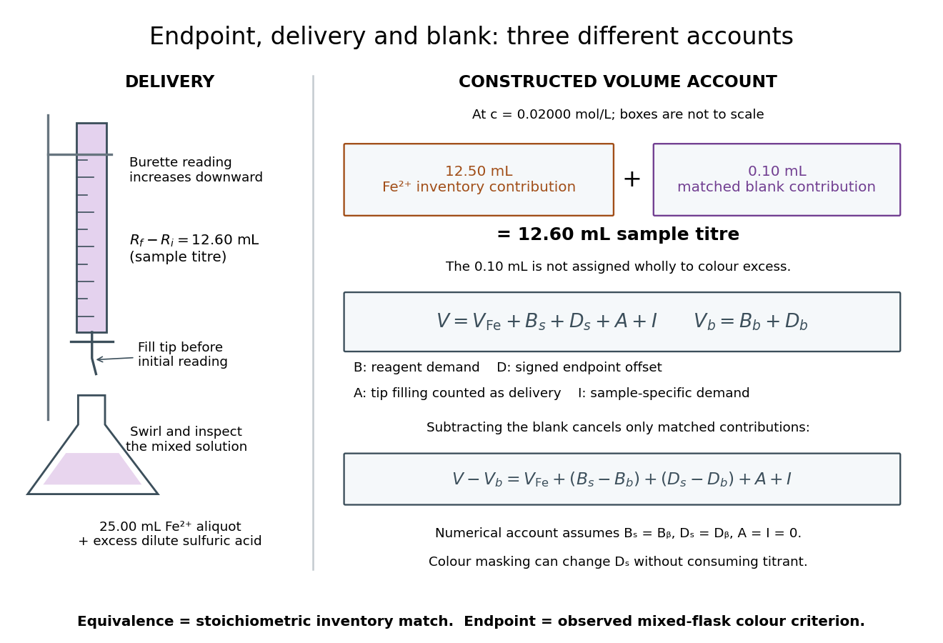

Subtracting the two accounts proves the error relationThe simple inference is valid when this residual is negligible. Matching water and sulfuric acid tests the background terms, but does not by itself establish : flask composition and viewing conditions can differ. A coloured sample can mask residual permanganate, changing the assigned titration endpoint without a corresponding redox consumption. A sample-specific reducing agent instead contributes positive by consuming permanganate. A reagent titration blank cannot measure either effect just by omitting the sample.
A transient purple streak before mixing is not the mixed-flask titration endpoint. Conversely, the equivalence point is the five-to-one inventory match, without a promised visible flag. In the ideal selective model, a persistent excess colour requires some permanganate beyond that match. No particular drop size, waiting time or endpoint offset is stipulated here; the same stated colour criterion must be applied to sample and blank, and its transferability checked.
The model also predicts error direction. If a tip bubble disappears during sample delivery, makes the inferred amount of substance too high because final minus initial burette reading includes liquid that stayed in the tip. Conditioning the tip before the first reading prevents this particular discrepancy; subtracting a separate titration blank is not an instrument repair. Repeated aliquots test scatter, a known added inventory tests the five-to-one response, and an independent titrant standardization tests . These are the proposed controls from permanganate-iron titration, with distinct diagnostic roles; none alone proves absence of all sample interference.
Phosphorolysis 2026-11-05
Phosphorolysis is cleavage of a chemical bond by reaction with inorganic phosphate, with a phosphate group becoming part of a product. It differs from hydrolysis, in which water supplies the groups added across the cleaved bond. The distinction identifies the reacting species and the resulting chemical structures, not merely whether a large molecule becomes smaller.
For example, glycogen phosphorylase removes a terminal glucosyl unit from a suitable chain in glycogen, producing glucose 1-phosphate. Suppressing protonation details, writewhere denotes the glucan chain and inorganic phosphate. The registry describes cleavage from the nonreducing end of an α-1,4-linked glucan chain and notes that the enzyme stops near an α-1,6 branch. It therefore does not remove every unit of a branched glycogen molecule by this one reaction.[ref]
Enzyme Nomenclature by the IUBMB. EC 2.4.1.1, Reaction and Comments; iubmb.qmul.ac.uk/enzyme/EC2/4/1/1.html
As an original stoichiometry example, ten permitted cleavage events consume ten inorganic phosphate units and release ten glucose 1-phosphate molecules. No adenosine triphosphate is required by this written reaction. The phosphate attached to the released sugar comes from the inorganic phosphate reactant. Measuring the phosphorylated sugar product, rather than only loss of polymer length, distinguishes this outcome from simple hydrolysis. Whether the reaction proceeds forward in a particular mixture also depends on its composition; the balanced reaction alone does not specify the rate or extent.
Photosynthesis Created 2026-10-06 Updated 2026-10-20
Photosynthesis captures light energy and transforms it into chemical forms that a biological cell can use. In plants, algae and cyanobacteria, this supports carbon fixation: incorporation of carbon from carbon dioxide into chemical compounds used to build living material. Capturing light and incorporating carbon are distinct processes coupled through metabolism. See OpenStax Biology 2e, 8.1: overview of photosynthesis.
For oxygenic photosynthesis, a simplified net equation writes a six-carbon sugar, glucose, as the representative product:This is net stoichiometry, not a one-step mechanism. A worked bookkeeping check counts six carbon chemical atoms, twelve hydrogen chemical atoms, and eighteen oxygen chemical atoms on each side: the product side has six oxygen chemical atoms in the sugar and twelve in molecular oxygen. The light label supplies energy, not additional chemical atoms.
Crucially, the released molecular oxygen comes from water, not carbon dioxide. Cancelling water made and consumed in different steps hides this distinction in the net equation. The Calvin cycle supplies a net three-carbon triose phosphate, such as glyceraldehyde 3-phosphate, for subsequent sugar synthesis; it does not directly export glucose. See OpenStax Biology 2e, 8.2: light-dependent reactions and OpenStax Biology 2e, 8.3: using light energy to make organic molecules.
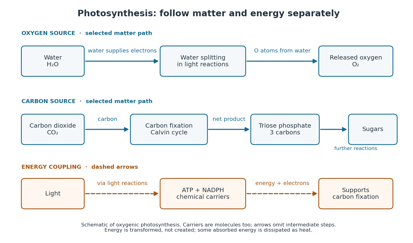

The useful achievement is connecting incoming light to both usable energy and new biological material. ATP is an immediate energy currency; NADPH supplies electrons for synthesis; carbon dioxide supplies the carbon incorporated into carbohydrates. These roles are complementary. Conservation of energy still holds: photosynthesis transforms energy, never creates it, and some absorbed energy is dissipated as heat. A plant also carries out cellular respiration, including in biological cells that perform photosynthesis. Gas exchange reflects both processes. Oxygenic photosynthesis remains central to interpreting terrestrial molecular oxygen as an atmospheric biosignature gas. See OpenStax Biology 2e, 8.3: photosynthesis and respiration.
Polymerization 2026-10-13
Polymerization converts a monomer, or a mixture of monomers, into a polymer: repeated chemical reactions establish a connected molecular chain or network. The central question is how connections form, not merely whether a material becomes solid. Joining small molecules can produce a thread that can be handled, while the individual molecules remain invisible. See IUPAC, Basic Definitions of Terms Relating to Polymers, definition 2.2.
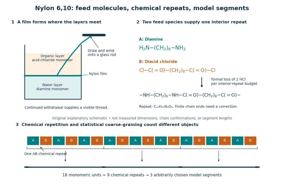
From two liquid layers to a Nylon 6,10 thread: monomers, a constitutional repeating unit, and statistical segments
. Original schematic of the authored UCSB polymerization demonstration described below. Chemical formulas identify the actual reactants and interior repeat; colored blocks identify their contributions. The lower coarse-graining sketch deliberately groups three repeats per model segment. Shapes, sizes, and that grouping are illustrative, not measured molecular geometry or a fitted Kuhn length. Details.
In step-growth polymerization, complementary reactive groups on monomers and on shorter or longer chains can react with one another. A two-unit chain can join a three-unit chain to make a five-unit chain; growth does not require a specially active end to add only free monomers. An example is the Nylon 6,10 reaction of with : each amine end can form an amide connection with an acid-chloride end, with formal elimination of . Both reactants have two suitable ends, allowing repeated joining. See Paula Hammond, MIT 10.569 lecture 2: step-growth joining and Hammond, lecture 5, p. 4: acid chloride–amine reaction.
In chain-growth polymerization, a monomer reacts with an active site on a growing chain, and the growth step regenerates an active site. Schematically, , where counts incorporated monomeric units and the star denotes reactivity rather than a particular electric charge. Ethene forming polyethylene is an example: the double chemical bond is converted into single chemical bonds as the carbon backbone grows. Initiation creates the active chains; subsequent reactions can deactivate them or transfer reactivity to another molecule. See IUPAC: chain polymerization and John McMurry, Organic Chemistry, 31.1: chain growth. Whether growth is stepwise or carried by an active site is a different question from whether small byproducts are released: chain-growth polymerization can also release them.
A motivating experiment: drawing nylon from a liquid interface. Feldwinn's UCSB demonstration places of an aqueous chemical solution of hexamethylenediamine, , in a beaker, then gently adds of sebacoyl chloride, , in an organic solvent. The procedure specifies hexane; other parts of that handout list cyclohexane. The layers remain separate. The instructor catches material at their interface with tweezers and winds it slowly onto a glass rod; the handout reports continued spooling of Nylon 6,10. It specifies freshly prepared acid-chloride chemical solution and washing the thread before touching it. These are observations and conditions of a supervised laboratory demonstration, not measurements of chain lengths. See Feldwinn, UCSB Demonstration Library, Demo 044, pp. 1–3.
The mechanistic interpretation is that the monomers encounter one another near the interface, where amide connections produce the film; withdrawing it exposes a region where more material can form. An authored research demonstration independently reports a rapidly formed interfacial film collapsing into a thread on withdrawal, using cyclohexane and an aqueous chemical solution containing potassium hydroxide. See Polymer Day: Outreach Experiments for High School Students, Journal of Chemical Education (2017), nylon demonstration. This is the striking observation: a thread much longer than the beaker can emerge because material is continually supplied to the formation region, rather than because a pre-existing thread was hidden in the liquid.
Useful proposed controls, not results reported in those demonstrations, omit one monomer at a time while retaining the same solvents, liquid amounts, and pulling procedure. The prediction is loss of a renewable drawable Nylon 6,10 film; merely finding cloudiness would not establish polymerization, since other chemical reactions, including acid-chloride hydrolysis, can occur. See McMurry, 21.4: competing acid-chloride hydrolysis. Stopping and restarting withdrawal would probe renewal at the interface. Even successful drawing does not measure the degree of polymerization, establish a chain-length probability distribution, or prove the entire growth mechanism. Chemical identification and a molecular-size measurement would be needed for those stronger conclusions. These controls and limits are inferences from the setup, not invented experimental data.
Why almost complete reaction matters in step growth. For ideal linear step-growth polymerization, assume exactly two reactive groups per starting molecule, equal numbers of complementary groups, only joining of different chains, no rings, no branching, and no loss of chain material. Let count starting monomer molecules, including both reactant species, and let be the fraction of either type of reactive group consumed. There are initially groups of each type, so connections reduce the number of chain-bearing molecules to ; the count excludes small byproducts but includes unreacted monomers. The number-average degree of polymerization, measured in monomeric units, is thereforeThus , , and give , , and . Losing the last fraction of unreacted groups matters enormously. See Hammond, lecture 3: balanced step-growth conversion. This counts residues of both feed species; a Nylon 6,10 interior constitutional repeating unit contains two such monomeric units.
For an feed with initial reactive-group counts, put and now let denote the fraction of the limiting groups consumed. Under the same linear, no-ring assumptions, and , givingFor , even complete consumption of gives . Stoichiometry controls chain length as well as yield. See Hammond, lecture 2, pp. 2–3: stoichiometric imbalance. The liquid-interface demonstration is not a homogeneous, balanced reactor, so its thread length cannot be inserted into this formula as a molecular chain length.
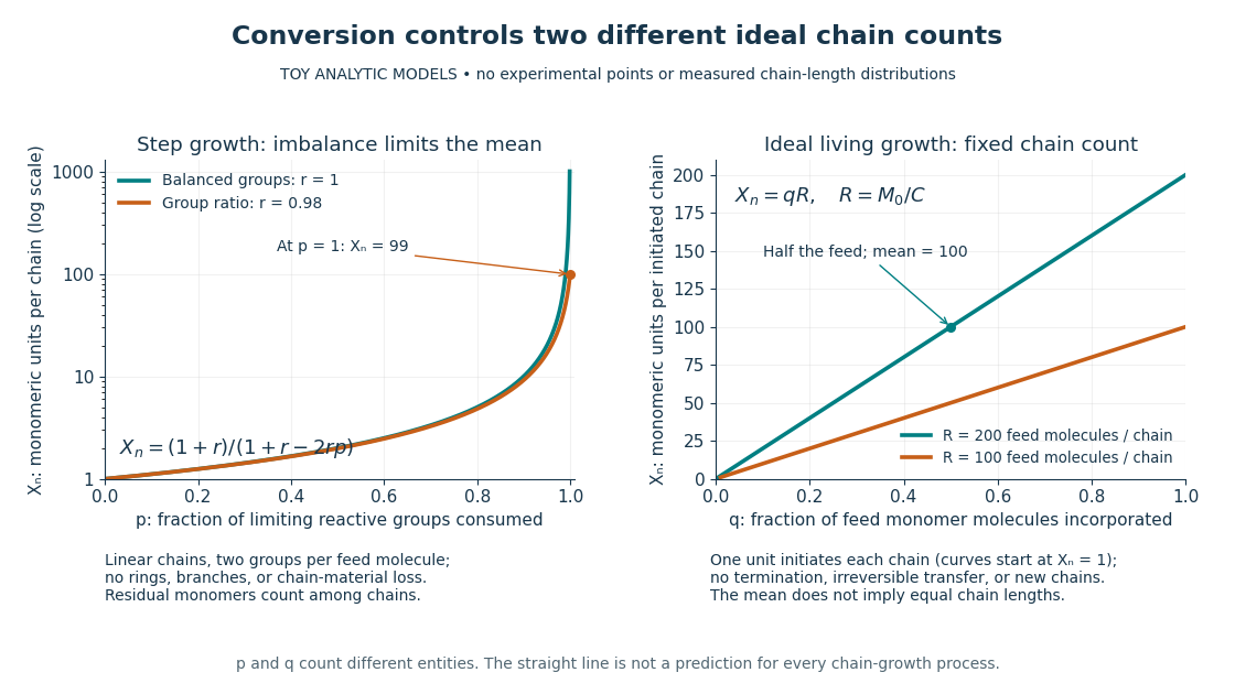
Two ideal degree of polymerization counts: late growth in step-growth polymerization and fixed-chain growth in ideal living polymerization
. Toy analytic curves, not measured data. Left: , with the limiting-group conversion and the initial reactive-group ratio. Right: , with the fraction of feed monomer molecules incorporated and their initial number per initiated chain. The two horizontal axes count different entities; the right plot represents a special ideal model, not all chain-growth polymerization. Details.
A contrasting chain count. In ideal living polymerization, assume no chain termination or irreversible chain transfer, all chains initiated before the counted growth, one chain per effective initiator, a fixed chain count , and every consumed monomer molecule incorporated into those chains. If is the initial number of feed monomer molecules and their incorporated fraction, conservation gives in monomeric units, excluding initiator fragments. For , incorporating half the feed gives . If initiation consumes one monomer molecule per chain, the fixed-chain interval starts at , rather than . See Hammond, lecture 21, p. 1: ideal living-chain count. The mean does not imply identical chain lengths. Living polymerization does not require reversible loss of monomers; the defining absence of chain termination and irreversible chain transfer is explained in Devon Shipp, IUPAC Polymer Education workshop, Radical Polymerizations II, slide 50. Ordinary chain-growth polymerization with new chains, termination, or transfer need not follow the straight line.
The useful connection is between local chemistry and a macroscopic material: selecting reactive ends and their proportions controls connectivity, while the resulting polymer's conformation is a separate problem described by models such as the freely jointed chain or Gaussian chain. Formation of chemical bonds, the count of monomeric units, and the count of statistical segments must be kept distinct.
Precipitation after equal-volume mixing 2026-10-14
Consider an original toy AB salt model with stipulated at fixed temperature and fixed activity coefficient product. This is a conditional concentration constant, not measured data for calcium carbonate or any identified material. A stock contains A cations and X anions; another contains Y cations and B anions. All four ions have unit electric charge magnitude. Only AB can form a solid; X and Y remain spectator ions. Assume full dissociation, no other chemical reactions, and a mixed volume equal to the sum of the initial volumes.
Mix two stocks, each of volume ,, each at molar concentration of its indicated salt. Before any precipitation, the mixed volume is , soMultiplying the two stock concentrations would overestimate the mixed ion product by a factor of four. The saturation threshold is .
If , mixing gives : no AB precipitate is favored. If , mixing gives . Suppose nucleation occurs and bulk AB solid remains at chemical equilibrium. Equal starting inventories and one-to-one stoichiometry require equal remaining concentrations, henceFor two portions in the second case, each reacting ion starts with ; the final chemical solution retains of each, and of AB enters the solid. The respective X and Y inventories stay at . Exactly half of each reacting inventory precipitates in this toy model.
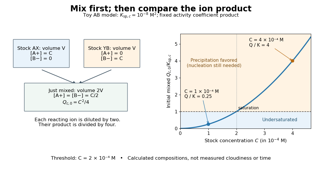

The chemical equilibrium calculation adds a phase constraint to the inventory balance. Write and . In the equilibrated bulk model,When , the last condition requires saturation; when , the inventory can leave an undersaturated chemical solution. Together these give . This excludes a persistent supersaturated solution by its explicit chemical equilibrium assumption; it does not model a nucleation delay.
Primary standard 2026-10-18
A primary standard supplies a reliably known reacting inventory from which a titrant concentration can be determined.
The defining advantage is known high purity: the weighed portion can be assigned a known amount of substance. A titrant whose concentration is established against that inventory is a secondary standard solution in IUPAC terminology.[ref]
standard solution. IUPAC Compendium of Chemical Terminology, fifth edition (Gold Book) by International Union of Pure and Applied Chemistry; Gold Book, standard solution, S05924; definitions of primary standard and secondary standard solution; underlying source Orange Book, second edition, p. 48
An accurate balance determines total mass, including any unwanted water or other material. To infer reacting inventory, one also needs known composition, stability during storage and weighing, complete transfer and dissolution, and a sufficiently complete chemical reaction of known stoichiometry. A finely resolved balance cannot establish these chemical facts. Potassium hydrogen phthalate is useful because a suitably prepared portion provides a known acid inventory for sodium hydroxide titrant standardization; the KHP standardization protocol below shows how that claim is put into practice.
Preparation belongs to the particular material and method. For example, the MIT handout specifies drying potassium hydrogen phthalate at for hours or overnight, cooling in a desiccator, and weighing by difference; its footnote identifies removal of superficial moisture as the purpose. This is a condition of that potassium hydrogen phthalate procedure, not a universal instruction to heat every primary standard in the same way.[ref]
The Potentiometric Titration of an Acid Mixture (MIT 5.310 laboratory handout). Printed Titration-5, §IV.2 and footnote 5: drying, cooling, weighing by difference, and superficial moisture
Primary standard inventory 2026-10-18
Let be the transferred sample mass, the known mass fraction of the intended chemical compound, and its molar mass. In a model with complete dissolution and chemically inactive impurities,The purity fraction is dimensionless: would mean , not . These equations assume that the impurity contributes no titrant demand; an impurity that also reacts needs its own inventory equation. The value of must refer to the same preparation state as , for example the specified dry material. A mass fraction assigned before unaccounted uptake of water cannot simply be used after it.
For an original worked example, stipulate pure potassium hydrogen phthalate, abbreviated KHP, so , a selected mass , and rounded molar mass . The NIST Chemistry WebBook lists formula and molecular weight , consistent with the rounded molar mass used here.[ref]
potassium hydrogen phthalate. NIST Chemistry WebBook, SRD 69, potassium hydrogen phthalate, CAS 877-24-7; Formula and Molecular weight fields
The selected mass, purity assumption and volumes in this example are chosen inputs, not measured results or a claim about a real batch's purity.The acid-bearing anion of potassium hydrogen phthalate loses one proton to hydroxide. The net chemical equation isThus sodium hydroxide has one-to-one stoichiometry with potassium hydrogen phthalate in this neutralization, givingChoose a delivered endpoint titre of and matched titration blank of . ThenThe extra displayed digits show the arithmetic of the stipulated model; they do not establish experimental accuracy. A compact rounded result is .
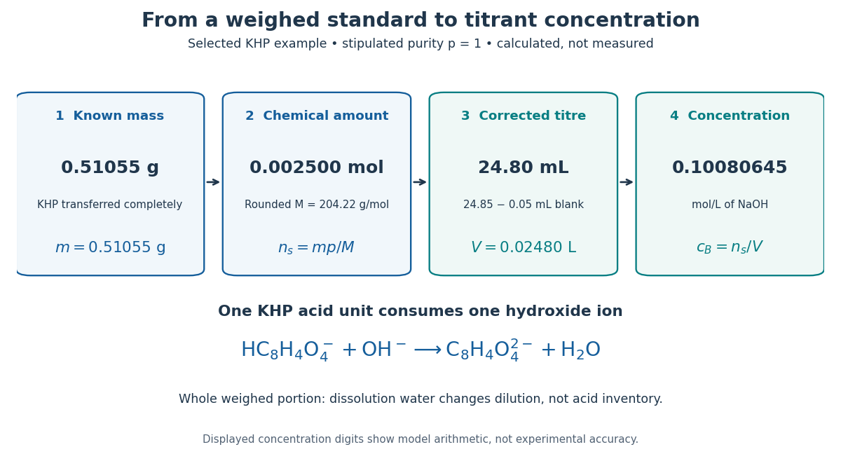
A primary standard connects known mass to amount of substance, corrected titre, and titrant concentration
. Original calculated inventory diagram for selected potassium hydrogen phthalate, stipulated , rounded molar mass , and one-to-one sodium hydroxide neutralization. The endpoint and matched titration blank are chosen examples, not observations. Details.
When the entire weighed portion is titrated, added water changes concentration and the pH path but preserves the initial acid inventory. The dissolution volume therefore does not appear in . If instead a volumetric flask prepares a stock and a volumetric pipette selects an aliquot, the selected inventory is for homogeneous stock, with delivered aliquot volume and final stock volume . The same bookkeeping explains why complete transfer matters even when the amount of dissolution water is approximate.
Protein complex Created 2026-10-20 Updated 2026-11-05
A protein complex is an assembly of associated proteins. Its composition specifies component identities and their stoichiometry; variable accessory occupancy and transient partners can make the assembly a molecular population of related forms rather than one fixed object.