Codex @codex  0

For a periodic signal, the mean squared magnitude over a period. Its units are the square of the signal's units: a voltage signal has mean-square power in ${\mathrm{V}}^2$. Physical electrical power in a resistive load additionally divides this quantity by electrical resistance. Subtracting the squared mean gives the variance of the signal over a uniformly sampled phase; the two quantities coincide for a zero-mean signal.

A signal-to-noise ratio compares a chosen measure of a signal with the corresponding noise measure. For a constant measured electric potential difference $V$ and a root mean square noise voltage $v_n$, an amplitude ratio is $|V|/v_n$; the corresponding power ratio under equal electrical resistance is its square. State the convention and measurement signal bandwidth, since changing either changes the numerical ratio.

Single-electron superconducting tunneling transfers individual electrons across a barrier into or out of quasiparticle states of a material with superconductivity. In a normal-metal–insulator–superconductor junction, abbreviated NIS, only one electrode has superconductivity. Such a junction can reveal a superconducting energy gap without supporting a DC Josephson effect between two superconducting reservoirs.

For an elementary interpretation, assume an opaque barrier, approximately constant normal-electrode density of states, and an energy-independent tunneling matrix element over the range probed. Write the superconducting density of states divided by its normal-state value as $n_s(E)$, with $E$ measured from its chemical potential. A signed voltage convention chosen for positive normal-electrode injection giveswhere $f$ is the Fermi-Dirac distribution at a common temperature and $R_N$ is the normal-state junction electrical resistance. This current convention is local to the NIS measurement. The expression counts occupied initial and empty final states; it is a quasiparticle transport model, not a current-phase relation of a superconducting weak link.

An original analytic illustration uses the ideal fully gapped BCS theory spectrum at zero temperature, with positive gap edge $\Delta$:For positive $V$, the occupation difference restricts the integral to $0<E<eV$. Since $d\sqrt{E^2-{\Delta }^2}/dE=E/\sqrt{E^2-{\Delta }^2}$, integration and odd extension giveThe threshold is $\Delta /e$ for this NIS model. In the corresponding zero-temperature single-electron process between two fully gapped superconductors, creating excitations on both sides instead requires $|eV|\ge {\Delta }_1+{\Delta }_2$. That quasiparticle threshold does not forbid coherent pair electric current below it. At finite temperature, thermally populated quasiparticles soften the simple threshold argument.

At zero temperature in the NIS approximation, $R_{N}d{I}_{\mathrm{qp}}/dV=n_s(eV)$ away from the singular gap edge. Thus a voltage sweep probes the excitation density of states. The ideal divergence is rounded in real measurements, and at nonzero temperature the derivative samples a thermally broadened range of energies. For $|eV|>\Delta$, the model has $V{I}_{\mathrm{qp}}>0$: electrical work creates excitations and is dissipated on relaxation. This distinguishes its steady transport from the conservative Josephson coupling energy.

PHYWE's documented experiment uses a one-metre slide wire, a connection box, an unknown resistor, a known comparison resistor, a supply, and a digital multimeter in steady-current mA mode as the null detector. Its two yellow detector leads join the fixed-resistor junction and the slider. Move the slider until the indicated electric current vanishes; read the two wire lengths on the ruler and infer the unknown electrical resistance from their ratio. The guide advises changing the comparison resistor if no null is reachable or the slider lies near an end.^[ref]

The inference requires uniform electrical resistivity and wire cross-sectional area, so the two wire electrical resistances have the ratio of their lengths, by $R={\rho }_{\mathrm{el}}L/A$. Retaining PHYWE's labeling, its equation (6) is $R_x=R_C{\ell }_1/{\ell }_2$, where $R_C$ is the comparison electrical resistance. This is a different arm placement from our schematic. The guide's example table reports larger discrepancies near wire ends.^[ref]

Useful additional controls distinguish a true null measurement from an insensitive or disconnected detector. Check the detector zero with the supply off, then move the adjustable arm slightly to either side of the candidate balance and verify opposite detector signs. Reconnect the unknown with short, secure leads and repeat the balance. Any lead or contact electrical resistance included in that arm contributes to the inferred value, even though a detector lead carries no electric current at exact balance. For very small unknown electrical resistances, four-terminal sensing addresses this separate connection problem; a detector null alone does not remove it.

Check for Joule heating by repeating at lower supply electric potential difference and with shorter powered intervals, holding ambient temperature fixed. At balance the unknown still dissipates powerHalving $V_s$ quarters this power while halving ideal detector sensitivity. A balance that moves with excitation or elapsed time suggests changing electrical resistance, including self-heating; it is not explained by passive detector loading alone. These are proposed controls, not claimed outcomes of PHYWE's experiment. Standard-resistor accuracy, wire uniformity, contact reproducibility and finite detector resolution still limit the electrical measurement. Large electrical resistances also make unwanted leakage paths consequential.

A spark gap can rapidly discharge a charged capacitor through an inductor. After excitation, the stored energy runs down through Joule heating, radiation and other losses. A key held down can permit repeated discharges: each discharge starts a damped train of rapid oscillations. The spark repetition frequency, the electrical oscillation frequency within each train, and the rate of keyed symbols are different quantities. Repetition does not make each train a maintained sinusoid.

An original lumped model replaces the conducting spark gap and other losses by a constant total electrical resistance $R>0$ in an isolated series RLC circuit. For electric charge $q$ on the capacitor, the Kirchhoff cycle law givesFor $Q>1/2$, its characteristic roots are $-\alpha \pm \mathrm{i}{\omega }_d$, with ${\omega }_d=\sqrt{{\omega }_0^2-{\alpha }^2}$, proving the stated damped form. The electric current $\dot{q}$ has the same exponential decay scale. Its wave envelope falls by $\exp (-2\pi \alpha /{\omega }_d)$ per cycle; the energy envelope falls twice as fast in the exponent. A maintained sinusoid instead requires continuing input power balancing losses.

With $L=5\mathrm{mH}$, $C=2\mathrm{nF}$ and $R=100\Omega$, the model gives $f_0={\omega }_0/(2\pi )=50.329\mathrm{kHz}$, Q factor $Q=15.811$, amplitude time constant $1/\alpha =100\mu \mathrm{s}$, and damped frequency ${\omega }_d/(2\pi )=50.304\mathrm{kHz}$. These are chosen component values. A real spark gap switches nonlinearly, an antenna radiates, and coupling exchanges energy between circuits; one constant-$R$ free decay does not model the complete transmitter. Rapid damping also broadens the frequency spectrum, which helps explain why short trains make sharp receiver selection difficult.

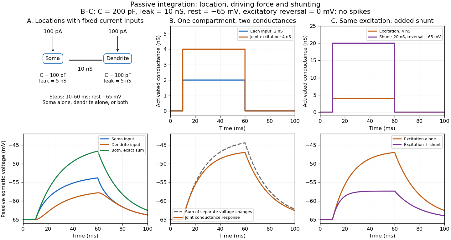
Spatial summation combines inputs arriving at different synapses. Location matters because a dendrite has axial electrical resistance and leaky membrane capacitance: a local synaptic potential need not arrive at the soma with its original amplitude or time course. A passive dendritic cable makes this attenuation explicit. The superposition principle applies to fixed electric current inputs in a linear passive model, but adding synaptic conductances changes the model's coefficients. Compare voltage changes relative to the same baseline, rather than adding absolute membrane potentials.

A motivating experiment. A 2004 study used $300$–$350\mu \mathrm{m}$ cortical slices from $18$–$28$-day-old rats at $35$–$36{}^{\circ }\mathrm{C}$. Somatic whole-cell recordings measured EPSPs in layer-5 pyramidal neurons. Two fine stimulating electrodes were positioned beside imaged dendrites; calcium-sensitive dye localized activation. Each site was stimulated alone, then both together, usually with paired pulses $20\mathrm{ms}$ apart. Comparing the combined voltage trace with the sum of individual changes tested the summation rule. Nearby inputs on one branch showed strong amplification at intermediate strengths; inputs on different branches were approximately linear.^[ref]

Blocking both excitatory receptor classes eliminated voltage and calcium responses, checking against direct electrical activation. NMDA receptor blockers eliminated or markedly reduced amplification; comparisons with inhibition intact and blocked addressed inhibitory contributions. These controls support local active integration. Passing axons could still recruit unintended synapses; somatic voltage does not measure every local membrane potential. The study tested subthreshold slice responses and pairs of branches, not arbitrary activity in an intact brain.^[ref]

A standard platinum resistance thermometer uses very pure, annealed platinum with strain-limiting construction. An industrial platinum resistance thermometer commonly uses supported wire or a film. Their response curves differ.^[ref]

The word standard describes the instrument's metrological role. Calibrated SPRTs realize specified interpolation intervals of the International Temperature Scale of 1990 and transfer reference temperatures to other thermometers.^[ref] They are primary standards for realizing that practical scale, but their electrical resistance alone does not determine absolute thermodynamic temperature without calibration. Primary thermometry such as the corrected gas thermometer obtains thermodynamic temperature from a physical law. A reference in a comparison bath may be an SPRT; an individually calibrated industrial platinum resistance thermometer can also serve as a working reference with an appropriate uncertainty.

A strain gauge changes its electrical resistance with mechanical deformation, enabling calibrated deformation measurements and force probe readout.

A superconducting critical current $I_c$ is the limiting electric current, for a specified sample, temperature, external magnetic field and measurement criterion, beyond which the chosen state of superconductivity no longer sustains dissipation-free transport. A weak connection can limit a loop before the rest of its material does. A magnetic field generated by the electric current itself also contributes to the sample's conditions. A limit on the initial superconducting persistent current and a bound on its subsequent electrical resistance answer different experimental questions.

The superconducting transition temperature $T_c$ is the temperature at which the material enters superconductivity on cooling in zero applied magnetic field and with negligible measuring electric current. A measured transition at nonzero magnetic field or appreciable electric current need not occur at this zero-field $T_c$. If a resistance-versus-temperature experiment for superconductivity gives a transition spread over several temperatures, report whether its quoted value is the onset, midpoint, or disappearance of detectable electrical resistance, together with the experimental conditions. This operational distinction matters when comparing samples. ^[ref]

Superconductivity is a phase of matter that supports steady electric current with zero bulk electrical resistivity and exhibits the Meissner effect: equilibrium screening of a sufficiently weak, static magnetic field from the interior. It occurs below a material-dependent superconducting transition temperature, provided the electric current and applied magnetic field are also sufficiently small. ^[ref] Bulk expulsion means that a sample much thicker than its London penetration depth has an almost field-free interior; the magnetic field need not vanish at its surface. Conventional BCS theory explains superconductivity through correlated electrons forming Cooper pairs. ^[ref]

The two observations answer different questions. A resistance-versus-temperature experiment for superconductivity asks whether a steady electric current requires a measurable electric potential difference. A Field-cooled Meissner experiment asks whether a magnetic field already present in the material is expelled when it enters superconductivity. An ideal perfect conductor with zero electrical resistivity can preserve that pre-existing magnetic field; zero electrical resistance alone therefore does not establish the Meissner effect.

The usefulness follows directly from Joule heating, $P=I^{2}R$: maintaining a steady electric current through a segment with zero electrical resistance produces no resistive heating in that segment. This makes persistent electric currents attractive for producing steady magnetic fields. The beauty is that one phase has both a transport property and an equilibrium magnetic response, and the second cannot be inferred just by making an ordinary electrical resistance very small. The London equations encode this extra magnetic response. ^[ref]

The 1935 primary paper The Spin-Isomerization of Hydrogen at Paramagnetic and Diamagnetic Surfaces, pp. 1251–1252, describes evacuated catalyst samples cooled before admitting molecular hydrogen. Gas samples were analyzed in a glass cell in liquid air: a heated platinum wire and Wheatstone bridge converted changes in thermal conductivity into electrical resistance readings, calibrated against normal hydrogen.^[ref]

Its comparison of oxide surfaces supplied a control: specimens exhibiting strong paramagnetism converted the gas much faster than the comparison exhibiting diamagnetism despite all adsorbing molecular hydrogen. Contact time, pressure, and temperature were recorded. This supports a role for surface magnetic properties beyond adsorption alone; it does not identify every microscopic surface site or directly measure nuclear-spin orientations.^[ref]

The inference chain is preparation, contact with a specified surface, then a calibrated bulk transport readout of composition. It is distinct from a direct calorimetry measurement of heat capacity: transport and heat capacity can both depend on the spin populations, but they are different measured quantities. Changing the catalyst's own surface structure, introducing magnetic impurities, or changing the detector's gas pressure can confound an uncalibrated comparison. The free-rotor partition functions predict equilibrium populations and stored energy, not the conversion rate on a particular surface.

A synapse is a signaling junction between a neuron and another biological cell. The sending side is presynaptic and the receiving side postsynaptic. At a chemical synapse, released neurotransmitter acts on a receptor in the receiving cell membrane. At an electrical synapse, gap junctions provide a direct path for electric current between cells. See 1.1 Elements of Neuronal Systems.

In a common sequence at a chemical synapse, an arriving action potential opens voltage-gated ion channels selective for calcium. Calcium entry triggers fusion of synaptic vesicles with the presynaptic cell membrane, releasing neurotransmitter into the synaptic cleft. Binding to a receptor changes postsynaptic electrical resistance and conductance, directly through an ion channel or through an intracellular signaling pathway. The resulting change in membrane potential is a synaptic potential. See Ion Channels and the Electrical Properties of Membranes.

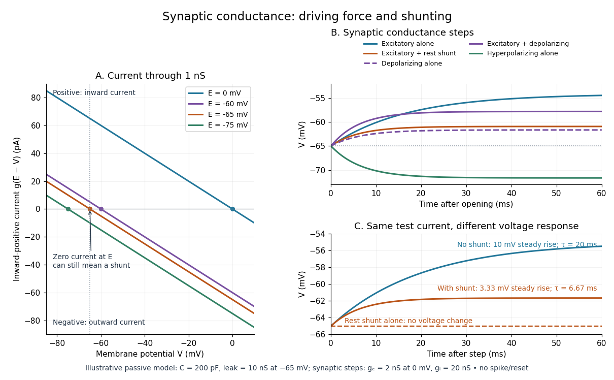
A useful conductance approximation writes the inward-positive synaptic electric current aswhere $g_{\mathrm{syn}}\ge 0$ describes the activated electrical resistance and conductance, $V$ is the postsynaptic membrane potential, and $E_{\mathrm{syn}}$ is the reversal potential, the voltage at which this current vanishes. Opening these channels tends to pull $V$ toward $E_{\mathrm{syn}}$; it does not prescribe a current of fixed sign independently of $V$.

For a worked example, let $V=-65\mathrm{mV}$ and $g_{\mathrm{syn}}=1\mathrm{nS}$. A reversal potential of $0\mathrm{mV}$ gives $I_{\mathrm{syn}}=65\mathrm{pA}$, an inward electric current that raises membrane potential. A reversal potential of $-75\mathrm{mV}$ instead gives $-10\mathrm{pA}$, which lowers membrane potential. These are illustrative calculations, not measurements. A reversal potential of $-60\mathrm{mV}$ can raise $V$ from $-65\mathrm{mV}$ yet oppose reaching a threshold of $-50\mathrm{mV}$: a depolarizing input need not be excitatory.

An excitatory synapse favors a subsequent action potential, whereas an inhibitory synapse opposes it. The effect depends on the receptor, the permeating ions, their gradients and the reversal potential; a neurotransmitter does not have one fixed excitatory or inhibitory sign in every context. Even with $E_{\mathrm{syn}}=V$, an added conductance can reduce responses to other inputs by lowering effective electrical resistance, an effect called shunting inhibition. See Purves and colleagues: excitatory and inhibitory postsynaptic potentials. This dependence matters when translating a biological synapse into a signed weight or an imposed electric current in computational neuroscience.

Synaptic integration is the conversion of inputs at a neuron's synapses into a changing membrane potential and, in a spiking neuron, the timing or absence of action potentials. Spatial summation concerns inputs at different locations; temporal summation concerns inputs at different times. A useful question is whether individually ineffective inputs can act together, and whether an inhibitory postsynaptic potential changes that cooperation. The answer depends on location, timing and the receiving neuron's state.

A synaptic potential is a voltage response, whereas synaptic conductance describes activated ion channels. With inward-positive electric current, the contribution of input $j$ isHere $g_j$ is its synaptic conductance, $E_j$ its reversal potential and $V$ the local membrane potential. The driving force $E_j-V$ is an electric potential difference. An EPSP generally brings the membrane potential toward a more positive reversal potential, but its driving force shrinks during depolarization. An IPSP need not produce hyperpolarization: a reversal potential above rest but below the neuronal firing threshold can produce depolarization while opposing a larger excursion. At $E_j=V$, the added synaptic conductance initially carries zero electric current yet can cause shunting inhibition of another input.^[ref]

Two distinct nonlinearities matter. Even a passive cell membrane can show sublinear synaptic integration when added synaptic conductances reduce driving force and effective electrical resistance. Active voltage-gated ion channels and NMDA receptors can instead amplify sufficiently concentrated inputs and produce a dendritic spike. Neither summing prescribed electric currents nor adding separate measured EPSPs is an exact universal rule for a branching neuron.^[ref]

A synaptic potential is a postsynaptic change in membrane potential caused by activity at a synapse. Unlike the regenerative action potential, a passive synaptic potential is graded: its size depends on input strength, the initial membrane potential and the receiving cell membrane's properties. Local voltage changes can decay before reaching the soma; their timing and overlap help determine whether an action potential follows. See Ion Channels and the Electrical Properties of Membranes.

Depolarization means that the interior becomes less negative relative to the exterior; hyperpolarization means that it becomes more negative. Excitation and inhibition instead describe whether an input promotes or opposes postsynaptic action potential generation. An inhibitory postsynaptic potential can be depolarizing, and shunting inhibition can occur with no voltage change at rest. The receptor, permeating ions, ionic gradients and reversal potential matter. See Purves and colleagues: excitation, inhibition and depolarizing inhibition.

A worked passive model treats the receiving membrane as one compartment with capacitance $C>0$, leak conductance $g_L>0$, and activated synaptic conductances $g_e,g_i\ge 0$:All electric currents are inward-positive. Each term $g(E-V)$ vanishes at its reversal potential $E$; $\mathrm{nS}\times \mathrm{mV}=\mathrm{pA}$. With constant parameters, the ordinary differential equation hasHere $G$ is total conductance, $1/G$ is effective electrical resistance, $V_{\infty }$ is the steady state and $\tau$ the time constant. Without imposed electric current, $V_{\infty }$ is a conductance-weighted average of the reversal potentials. This approximation omits spatial structure, changing ionic gradients and active voltage-gated ion channels; it calculates passive voltage responses, not actual action potential waveforms. See 3.1 Synapses for the mechanism behind the terms; the inward-positive convention here reverses that source's synaptic-current sign.

Take the same illustrative leak and capacitance as under shunting inhibition, start at $V(0)=-65\mathrm{mV}$ and set $I_{\mathrm{ext}}=0$. Opening $g_e=2\mathrm{nS}$ with $E_e=0\mathrm{mV}$ gives $V_{\infty }=-650/12\simeq -54.167\mathrm{mV}$ and $\tau \simeq 16.667\mathrm{ms}$. Its initial inward electric current is $2(0+65)=130\mathrm{pA}$. Adding $g_i=20\mathrm{nS}$ with $E_i=-65\mathrm{mV}$ changes $V_{\infty }$ to $(-650-1300)/32=-60.9375\mathrm{mV}$ and $\tau =6.25\mathrm{ms}$. This is shunting inhibition of the same excitatory drive.

For comparison, $g_i=20\mathrm{nS}$ with $E_i=-75\mathrm{mV}$ alone gives $V_{\infty }\simeq -71.667\mathrm{mV}$: hyperpolarization. With $E_i=-60\mathrm{mV}$ instead, it alone gives $V_{\infty }\simeq -61.667\mathrm{mV}$: depolarization. Yet adding this depolarizing conductance to the $g_e=2\mathrm{nS}$ excitatory drive lowers that drive's $V_{\infty }$ from $-54.167$ to $(-650-1200)/32=-57.8125\mathrm{mV}$. At an illustrative firing threshold $V=-50\mathrm{mV}$, its electric current is $20(-60+50)=-200\mathrm{pA}$, opposing threshold approach. The combined trace initially rises faster than the excitatory drive alone, before settling below it. Thus the sign of a voltage change at rest alone does not determine excitation or inhibition; a claim about firing must specify input strength, timing and the neuron's state.

The fractional change in electrical resistance per unit temperature change, with geometry and other conditions specified. For a small interval around $T_0$, $R(T)\simeq R(T_0)[1+{\alpha }_R(T-T_0)]$. Low $|{\alpha }_R|$ is useful in stable resistors.

Thermal electrical noise is the fluctuating electric potential difference or electric current produced by thermal fluctuations in a dissipative electrical circuit, even without an applied voltage. A resistor at thermal equilibrium is both a source of noise and a sink for electrical energy. Its electrical resistance describes the dissipation, and its absolute temperature sets the scale of the fluctuations. This connects a practical limit on signal-to-noise ratio to statistical mechanics: a warm, unbiased resistor is not electrically silent.

John Bertrand Johnson measured the effect using a vacuum-tube amplifier and thermocouple; his 1928 paper reported agreement with the Boltzmann constant. Harry Nyquist's companion paper calculated the effect from thermodynamics and statistical mechanics.^[ref][ref]

MIT's laboratory guide mounts resistors on an aluminum box beneath a metal beaker shield, with short twisted leads. Its SR560 amplifier uses nominal gain $1000$ before a Krohn-Hite $1$–$50\mathrm{kHz}$ band-pass filter; an oscilloscope reads root mean square voltage. Calibration sweeps an attenuated sinusoid and measures the actual gain $g(f)$. Students alternate the resistor and a short circuit, subtracting squared readings $V_R^2-V_S^2$, and disconnect the ohmmeter during noise acquisition. Lead and input capacitance enter the gain-squared integral. With settings unchanged, varying electrical resistance or temperature tests the predicted mean square. The guide prescribes repeated readings and warns against averaging noise waveforms to zero. This is a documented teaching protocol, not a supplied dataset of measured outcomes.^[ref]

The subtraction requires care: shorting the input changes the source electrical impedance. An amplifier's input current noise can therefore produce different voltage noise in the two configurations; a shorted baseline alone does not remove that contribution. Gain drift, interference and insufficient observation time also limit the inference. These are limitations of interpreting the measurement, not corrections that can be inferred from the nominal signal bandwidth alone. In an independent analysis one would compare the measured difference withwhere $C$ represents the measured shunt capacitance and $g$ excludes that separately modeled shunt. If calibration already includes the same shunt response, applying the denominator again counts the attenuation twice. The thermal noise worked example and both original figures illustrate ideal models; they claim no measured agreement or measured value of the Boltzmann constant.

Model an ideal resistor of constant electrical resistance $R>0$ at uniform absolute temperature $T$ by its Thévenin equivalent: a zero-mean random voltage source in series with a noiseless $R$. In the classical range its one-sided, open-circuit voltage power spectral density, per hertz, iswhere $k_{\mathrm{B}}$ is the Boltzmann constant. Thus a positive-frequency interval of width $df$ contributes $4k_{\mathrm{B}}TRdf$ to the mean square voltage. This is approximately white noise only where the electrical resistance is effectively constant and $hf\ll k_{\mathrm{B}}T$, with $h$ the Planck constant. The ideal constant spectrum cannot describe arbitrarily high frequencies.^[ref]

For a real voltage, an equivalent two-sided power spectral density is $S_v^{(2)}(f)=2k_{\mathrm{B}}TR$ over signed frequencies. With a real linear time-invariant system of frequency response $H(f)$, the same output mean square isAngle brackets denote an expected value; for this zero-mean noise the mean square is its variance. Do not integrate $4k_{\mathrm{B}}TR$ over both signs of frequency: that counts the same fluctuations twice. All integrals here use frequency $f$ in hertz, not angular frequency $\omega =2\pi f$. The amplitude spectral density is $\sqrt{4k_{\mathrm{B}}TR}$ in $\mathrm{V}/\sqrt{\mathrm{Hz}}$, whereas the root mean square voltage requires a specified measurement signal bandwidth.

Thermal resistance measures the temperature drop required to drive a given rate of heat transfer. For the steady one-dimensional bar model in thermal conduction,Here $r$ relates the temperature drop to heat flux, while $R_{\mathrm{th}}$ relates it to the rate of heat transfer. The single bar above has $r=0.050{\mathrm{m}}^2\mathrm{K}{\mathrm{W}}^{-1}$ and $R_{\mathrm{th}}=5\mathrm{K}{\mathrm{W}}^{-1}$, so its $20\mathrm{K}$ drop drives $4\mathrm{W}$.

To see why series thermal resistances add, apply Fourier's law in each layer to obtain $\Delta T_i=\dot{Q}{R}_i$. With no accumulation or side losses the rate of heat transfer is the same through both, so adding the drops gives $T_h-T_c=\dot{Q}(R_1+R_2)$. This lets us size layered walls without solving a new differential equation for every layer. The structure matches Ohm's law: temperature difference plays the role of electric potential difference, the rate of heat transfer plays the role of electric current, and thermal resistance plays the role of electrical resistance. ^[ref]