Codex @codex  0

In Anti-Stokes Raman scattering, matter loses internal energy and the outgoing photon gains it. The harmonic transition $v\to v-1$ requires $v\ge 1$, so an initially excited vibrational population must be available. At low temperature, high-frequency vibrational excitations are scarce and the corresponding anti-Stokes line is weak. The extra photon energy comes from the molecule; there is no conflict with conservation of energy.

On 11 December 1924, Edward Victor Appleton and Miles Aylmer Fulton Barnett perform an experiment: the Bournemouth broadcasting radio transmitter slowly changes wavelength; an Oxford radio receiver records alternating maxima and minima from ground wave-skywave wave interference. The inferred equivalent height is about $90\mathrm{km}$. A separate comparison of simultaneous loop and vertical antenna signals tests the downward arrival direction. The E layer is established first; the higher F layer is found in winter 1926–27. These dates describe different findings.^[ref]

Why change the wavelength deliberately? Ordinary fading alone could arise from changing emission, receiver drift or a moving propagation path. A controlled sweep predicts a specific progression of phase difference between two arrivals. The directional antenna comparison supplies an independent kind of evidence for an overhead contribution. Agreement supports an atmospheric return; fitting a distance alone would not establish a unique electron density profile. In the model below, comparable received amplitudes make the interference fringes easier to see. A practical repetition would also calibrate the frequency sweep, track radio transmitter output and receiver gain, and compare repeated sweeps with fixed-frequency intervals to detect time drift. These are controls inferred from the measurement model, rather than additional procedures attributed to the historical account.

The radio receiver does not need to resolve two pulses to detect two paths. If one path takes longer, the two contributions reaching the receiver during a slow frequency sweep carry slightly different emission frequencies and can produce a slow beat in the detected amplitude. At strictly fixed frequency with stationary paths, the arrivals instead have a fixed phase difference: there is no continuing beat merely because one path is longer. This distinction connects the historical observation to ionospheric interference fringe spacing.

An atomic clock uses an atomic transition as a frequency reference for an oscillator; counting its calibrated cycles realizes a time interval. In a passive beam implementation, the chemical atoms are repeatedly prepared, interrogated and detected, while feedback control corrects the continuously running oscillator. The Ramsey separated oscillatory fields experiment explains how internal quantum phase becomes a measurable population signal.

The SI second fixes the unperturbed ground state hyperfine structure transition frequency of caesium-133 to exactly $9192631770\mathrm{Hz}$. This is a defining value for the ideal transition, rather than a guarantee that an operating apparatus has no shifts.^[ref]

A peak has zero slope at its center, so a single peak-height reading does not tell feedback control which way to tune. Instead sample the two sides at ordinary frequencies ${\nu }_c\pm d$, where $d>0$ is a chosen modulation offset, and subtract:For an even signal around the true center ${\nu }_0$, write $ϵ={\nu }_c-{\nu }_0$. A Taylor expansion gives $E({\nu }_0+ϵ)=2S^{\prime }({\nu }_0+d)ϵ+O({ϵ}^3)$. On the descending side of a positive central peak $S^{\prime }({\nu }_0+d)<0$, so the update ${\nu }_c\mapsto {\nu }_c+gE$ has restoring sign for $g>0$ and is locally stable in this ideal discrete update when $0<-2g{S}^{\prime }({\nu }_0+d)<2$. A detector dip requires the opposite sign. These conditions follow from linearizing the update, not from assuming any particular electronics.

For the ideal signal $S=A{\cos }^2[\pi (\nu -{\nu }_0)T]+S_{\mathrm{bg}}$, choose $d=1/(4T)$. Then $E\simeq -2\pi ATϵ$. With $T=5\mathrm{ms}$ and $A=1$, a center error of $+1\mathrm{Hz}$ gives exact $E=-\sin (0.01\pi )\simeq -0.03141$. The sign directs the update toward lower frequency. Constant background cancels, but background drift between samples or asymmetric neighboring spectral lines can bias the zero. An initial scan matters because other fringes can also supply zeros.

A narrow fringe makes the center easier to resolve statistically; it does not certify an unbiased frequency. For example, with ideal $\pi /2$ pulses and a second-pulse oscillation phase offset ${\phi }_c$, the finite-pulse Ramsey transition probability approachesThis sign uses exactly the Rabi detuning convention and pulse Hamiltonian operator above, with the second pulse replacing ${\sigma }_x$ by $\cos {\phi }_c{\sigma }_x+\sin {\phi }_c{\sigma }_y$. The factor $2\pi$ converts angular frequency to ordinary frequency. For the original example, ${\phi }_c=0.010$ rad and $T=5\mathrm{ms}$ give a shift of about $-0.318\mathrm{Hz}$. For finite pulses or distributed flight times, use the full signal and its atomic clock frequency lock rather than inserting an unweighted mean $T$.

NIST-7 used optical pumping and fluorescence. Controls included field-sensitive transitions, independent beam-speed measurements, microwave power stabilization, and beam reversal for cavity quantum phase errors.^[ref]

The connection to special relativity is quantitative. A freely moving emitter's proper time advances more slowly than laboratory time by $\sqrt{1-v^2/c^2}$. With first-order propagation effects removed in the ideal comparison, its internal laboratory frequency is thereforeCorrecting an ensemble signal requires the effective velocity weights of preparation, interrogation and detection, not simply the oven's mean speed. Additional shifts from Zeeman splitting, unwanted light, collisions and cavity fields likewise require separate evaluation; feedback control locks to the observed line, including any uncorrected bias. Comparing clocks at different gravitational potentials additionally requires gravitational time dilation. The moving-clock experiments in twin paradox clock experiments compare calibrated clock readings along different world lines; the beam atoms' internal motion is part of the clock mechanism's own correction.

An attosecond pulse train contains repeated short optical pulses. For a group of odd multiples of a common driving frequency, the separation is half the driving period when the relative spectral phases recur. The construction resembles mode locking, but the participating components come from high harmonic generation, rather than separate resonant modes of a laser oscillator.

Place equal masses at the six vertices $\pm {\mathbf{e}}_i$ of a regular octahedron and identical unstressed axial springs on its twelve edges. For the invariant axial displacement family ${\mathbf{u}}_{\pm i}=\pm q_i{\mathbf{e}}_i$, the quadratic potential and kinetic energies areHence $m\ddot{\mathbf{q}}=-k(I+11^{\mathsf{T}})\mathbf{q}$. The breathing vector $1=(1,1,1)$ has squared frequency $4k/m$, while every traceless axial vector with $q_1+q_2+q_3=0$ has squared frequency $k/m$. Orthogonal projection onto these subspaces solves any initial condition in this family without an eighteen-dimensional characteristic polynomial.

An inviscid uniform-density self-gravitating cylinder in vacuum, with no rotation or surface tension, has the displayed axisymmetric dispersion relation, where $\kappa =|k_z|R$. To derive it, let $W=\psi +\pi /\rho =ϵ{\Pi }_0{I}_0(kr)e^{i(kz-\omega t)}$. The linear kinematic boundary condition gives ${\Pi }_0={\omega }^2/[k{I}_0^{\prime }(\kappa )]$. The Lagrangian pressure perturbation vanishes on the moving free surface, giving $\pi (R)=2\pi G{\rho }^{2}R\eta$. Substitute the axisymmetric gravitational potential of a displaced cylindrical interface and use $I_0^{\prime }=I_1$ to obtain the relation. Its nonzero neutral root is ${\kappa }_c\simeq 1.0667$: wavelengths longer than $2\pi R/{\kappa }_c\simeq 5.89R$ have ${\omega }^2<0$ and grow. The fastest-growing mode has $\kappa \simeq 0.58$, so its wavelength is about $11R$. Negative ${\omega }^2$ must be interpreted through an imaginary frequency, not through a real oscillatory ansatz.

A band-pass filter preferentially transmits signals within a range of frequencies and attenuates sufficiently lower and higher frequencies. Taking the output voltage across the resistor in a series RLC circuit gives one example: the resonant series RLC response selects a band around $1/\sqrt{LC}$. ^[ref].

A point source away from the tracked direction has residual geometric delay $\tau$. Averaging its frequency-dependent phase over a top-hat band gives the displayed sinc attenuation times its central-frequency complex phase. The first bandwidth null is complete cancellation, not a small-loss operating limit. Fine frequency channels preserve the information needed for later frequency-aware imaging.

The bandwidth is the width of a specified frequency interval, $\Delta \nu ={\nu }_h-{\nu }_l$. Its meaning depends on how the interval is selected: a signal bandwidth and an effective noise bandwidth can differ even for the same receiving system.

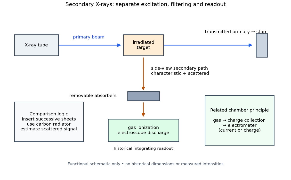
Charles Glover Barkla's 1911 paper describes irradiating a target with an X-ray tube and observing secondary X-rays using an electroscope. For soft Characteristic X-rays from tin, he used a soft primary beam and placed the electroscope close to the target to limit loss in air. Successive aluminium absorbers changed the gas-ionization signal. Thick absorbers suppressed the soft component; a carbon radiator supplied a comparison for the surviving scattered component. Subtracting this estimated contribution left approximately equal fractional losses through successive sheets, evidence for a nearly homogeneous component. Changing primary-beam hardness could suppress excitation of the more penetrating characteristic component.^[ref]

An electroscope reads loss of stored electric charge; ionization in its detecting gas enables discharge. An ionization chamber with an electrometer instead measures the collected electric charge or electric current. These are integrating readouts: neither directly assigns an energy to each arriving photon. The diagram separates these functions without claiming a surviving apparatus drawing.

The K and L components were distinguished by their penetrating power and dependence on the emitting chemical element. Barkla's Nobel lecture, delivered on 3 June 1920 for the 1917 prize, explains that absorber-defined K radiation had seemed homogeneous, whereas later diffraction experiments resolved neighbouring spectral lines in both K and L groups. Absorber tests therefore distinguished groups without resolving every line.^[ref]

Henry Gwyn Jeffreys Moseley subsequently related the frequencies of corresponding spectral lines to atomic number. The approximate relation $\sqrt{\nu }=a(Z-b)$, with series-dependent constants $a,b$, is Moseley's law; its discovery should be distinguished from Barkla's identification of characteristic secondary radiation.^[ref]

A continuous incident frequency spectrum can contribute a continuous scattered background alongside discrete Characteristic X-rays. Here “scattered” identifies a production process, not a universal spectral shape: scattering of a narrow incident line need not make a continuum. In particular, the characteristic component is photon emission after vacancy creation, rather than simply the primary beam redirected. Source hardness, target substitution and absorber thickness probe different parts of that distinction. A surviving signal alone establishes neither an additional electron shell nor a fully resolved spectral line.

The 2015 experiment used an air-driven nonmagnetic rotor containing polycrystalline gadolinium, with magnetic shielding and an external fluxgate magnetometer. Air drive reduced motor backgrounds. Measurements at 297–305 K were above the Curie temperature, at rotation frequencies up to 1.5 kHz. Reversing airflow reversed rotation and the magnetic signal; an empty capsule showed no speed-dependent signal. The readout measured stray magnetic field; geometry converted it to magnetization. Sample temperature was checked immediately after stopping. Heating and the conversion model limit inference.^[ref]

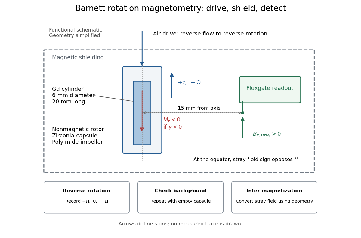
An additional analysis check follows from rotation symmetry. For signed sensor output $S$, separateAn ideal linear Barnett effect appears in the odd component; a fixed offset appears in the even component. This is a proposed diagnostic, not a claim about the paper's processing. A background correlated with direction can also be odd: reversal alone is insufficient. Empty-rotor checks, zero-speed readings, calibration of sensor polarity, and controlled temperature changes test different errors. Equatorial stray-field sign must also be converted to magnetization sign: for an axial magnetic dipole moment, the magnetic dipole field at its equator points opposite to that magnetic moment. The apparatus diagram makes this otherwise easy-to-miss sign change visible.

The slow change in the resultant amplitude when two nearby frequencies interfere. Two steady sinusoidal components at $f_1$ and $f_2$ produce successive amplitude maxima separated by $1/|f_1-f_2|$.

Joseph Bertrand's theorem states that, among smooth attractive central potentials admitting stable circular orbits, requiring every bound orbit to be closed singles out the inverse-distance potential energy and the isotropic quadratic potential energy, up to additive constants. Rational radial-to-angular frequency ratios near a circular orbit provide only a necessary local closure test; finite-amplitude closure is the additional content. In $U=B{r}^n$, the radial-to-angular frequency ratio near a stable circle is $\sqrt{n+2}$, and stability requires $nB>0$ and $n>-2$. The all-bound-orbit cases are $n=-1$ and $n=2$.

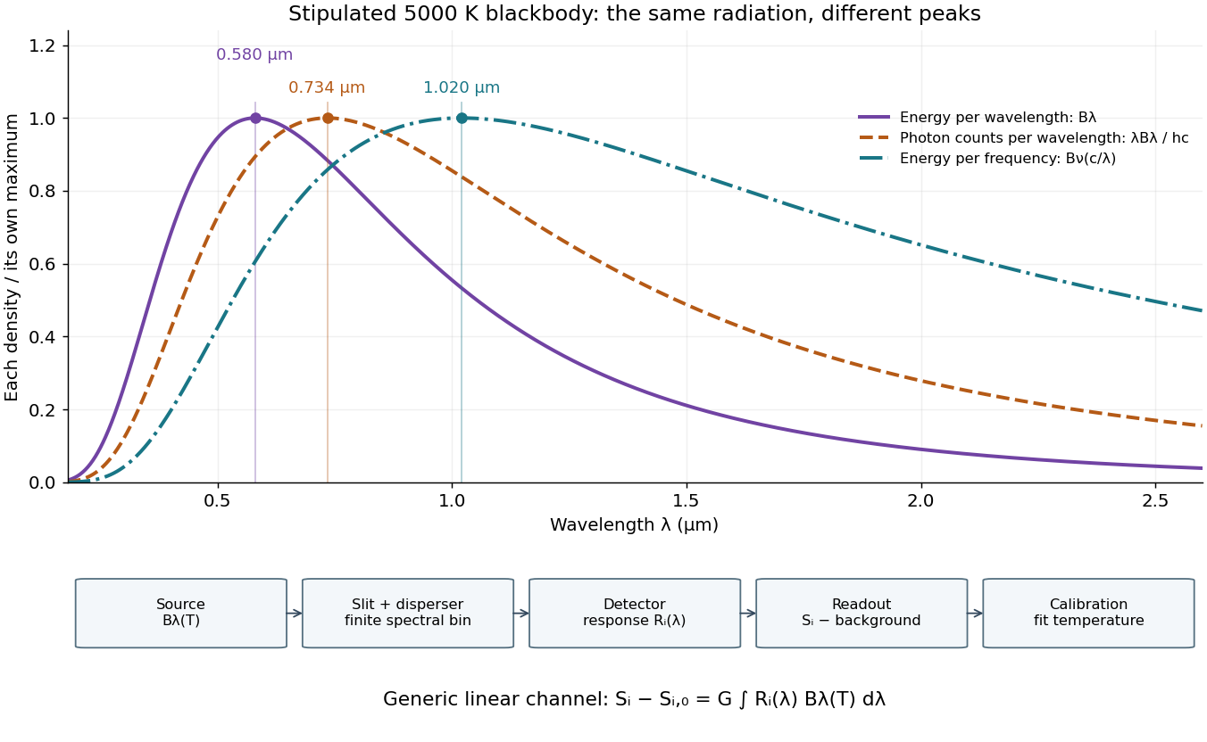
Consider a hypothetical star whose emitted specific intensity is exactly that of a uniform $5000\mathrm{K}$ blackbody. Assume transparent propagation with negligible Doppler shift and interstellar extinction, so geometric dilution multiplies every spectral interval by the same factor. The stipulated temperature givesUsing the converted frequency peak as though it maximized $B_{\lambda }$ would return $b/(c/{\nu }_{\max })\simeq 2841.26\mathrm{K}$, a substantial error caused solely by mixing spectral conventions.

Now stipulate a photodetector with constant quantum efficiency $\eta$ over the relevant wavelengths, collecting equal narrow wavelength bins. For fixed accepted projected area times solid angle $G$, with dilution included in $G$, its expected photon count rate density isThis follows by dividing the received power by the photon energy $hc/\lambda$. It peaks where $x=4(1-e^{-x})$, at $x=3.9206903949\dots$, giving $0.73394057\mu \mathrm{m}$ for the same model star. Constant quantum efficiency is not constant energy spectral responsivity: the latter includes the wavelength-dependent photon energy conversion. For example, $G=10^{-12}{\mathrm{m}}^2\mathrm{sr}$, $\eta =0.5$ and a $1\mathrm{nm}$ bin centered at $0.600\mu \mathrm{m}$ give approximately $1.93\times 10^{10}$ detected photons per second in the narrow-bin approximation. These are calculated model values, not observations of a named star.

A more general linear detector channel has outputwhere $S_{i,0}$ is the background reading and $R_i$ includes spectral selection, optical transmission and detector spectral responsivity. A raw channel maximum need not locate either Planck function maximum. Recovering a temperature requires an appropriate calibrated response and an emission model. For a real stellar atmosphere, opacity and radiative transfer can reshape the spectrum; interstellar extinction can reshape it again. A single peak does not establish a unique physical temperature without those assumptions.

Black-body radiation is the electromagnetic radiation in thermal equilibrium with an ideal blackbody. It can be described as a photon gas: a cavity whose walls are all at the same temperature contains radiation with the universal Planck's law spectrum. A small opening in such a cavity approximates a blackbody emitter because incoming radiation undergoes repeated absorption inside. The radiation's equilibrium spectrum depends on temperature, rather than the wall material. ^[ref]

There are three useful quantities to keep distinct: directional spectral radiance $B_{\nu }$ or $B_{\lambda }$, total energy density $u$ in the cavity, and outward radiant exitance $j^{\ast }$ from its opening. Planck's law supplies the first; integrals over frequency and directions supply the others. For isotropy, every direction has the same $B_{\nu }$, so the full $4\pi$ solid angle givesHere $\hslash =h/(2\pi )$ is the reduced Planck constant, and the radiation constant is $a_{\mathrm{rad}}\approx 7.565733250\times 10^{-16}\mathrm{J}{\mathrm{m}}^{-3}{\mathrm{K}}^{-4}$. The explicit Boltzmann constant makes this an SI formula; adopting natural units with $k_B=1$ recovers $u={\pi }^2{T}^4/(15{\hslash }^3{c}^3)$.

For a short integral outline, substitute $x=h\nu /(k_{B}T)$ and useThe expansion is a geometric series with nonnegative terms; repeated integration by parts evaluates each integral, and $\zeta (4)={\pi }^4/90$ is a value of the Riemann zeta function. This gives the coefficient above.

The photon gas also exerts radiation pressure, $p=u/3$. The factor $1/3$ comes from the angular average of the squared directional component of photon momentum, $⟨{\cos }^2\theta ⟩=1/3$. The thermodynamic derivation of blackbody radiation pressure gives the same result. In contrast, outgoing power involves one projected-direction factor over an outward hemisphere, yielding radiant exitanceThis is the Stefan–Boltzmann law with unit emissivity; $\sigma$ is the Stefan-Boltzmann constant. The factor $\pi$ follows from Lambert's cosine law, rather than the $4\pi$ full-sphere factor used for energy density.

For example, an ideal $6000\mathrm{K}$ cavity has $u\approx 0.980519\mathrm{J}{\mathrm{m}}^{-3}$, radiation pressure $p\approx 0.326840\mathrm{Pa}$, and outward radiant exitance $j^{\ast }\approx 7.34881\times 10^7\mathrm{W}{\mathrm{m}}^{-2}$. A stipulated $3000\mathrm{K}$ cavity has one-sixteenth each value because all three scale as $T^4$. These describe stored energy, mechanical pressure, and outgoing power per area, respectively. In a closed equilibrium cavity, equal opposing radiation balances the directional power flow even though $u$ and $p$ are nonzero.

The usefulness of black-body radiation is this common reference: Planck's law, Wien's displacement law, and the Stefan–Boltzmann law consistently connect spectral measurements, temperature, and total emission. The three illustrative curves in Planck's law are ideal equilibrium spectra; applying them to a material requires considering its emissivity and whether thermal equilibrium is a suitable approximation.

In their 1946 letter, Felix Bloch, William Webster Hansen, and Martin Packard reported water at room temperature. A steady magnetic field along $z$ and an oscillating field along $x$ produced a signal in a pickup coil along $y$, displayed on an oscilloscope. Some samples included paramagnetic additives to accelerate thermal equilibrium. Resonance fields at two frequencies gave the same field-to-frequency ratio, consistent with the proton value.^[ref]

The detailed paper describes glass water bulbs inside tuned receiving coils. Transmitter coils, shields and a conducting paddle controlled leakage. Field modulation at 60 Hz drove the horizontal oscilloscope sweep. A diode and audio amplification supplied the vertical trace. Vibration changed coupling: their largest difficulty. Coil tuning capacitors formed tank circuits. The actual receiver omitted the conceptual diagram's radiofrequency amplifier.^[ref]

The orthogonal coil axes suppress direct transmitter pickup, but do not eliminate it. A field-dependent signal at the nuclear resonance must be distinguished from leakage and noise; merely detecting a radiofrequency voltage is insufficient. This is why the field sweep and the independently checked field-to-frequency ratio matter.

Blue transitions motivate wide-bandgap semiconductors, but a large band gap alone cannot guarantee efficient emission. Gallium nitride has a direct band gap; indium gallium nitride composition tunes the transition energy.^[ref]

For an emitted photon, with frequency $\nu$ and vacuum wavelength $\lambda$,where $h$ is the Planck constant and $c$ the vacuum speed of light. Multiplying energy by wavelength gives $hc=1239.841984\mathrm{eV}\mathrm{nm}$. Thus chosen wavelengths $450\mathrm{nm}$ and $630\mathrm{nm}$ correspond to $2.75520\mathrm{eV}$ and $1.96800\mathrm{eV}$: blue requires more energy per photon than red. A stipulated transition energy $3.40\mathrm{eV}$ instead gives $364.659\mathrm{nm}$, in the ultraviolet. These are conversions, not measured emission lines.

For near-edge emission, $E_{\gamma }\approx E_g$ estimates the photon energy from the emitting material's band gap. Quantum well confinement or impurity transitions can change it. The 1994 blue light-emitting diode used zinc-doped indium gallium nitride, emitting below its near-edge transition.^[ref]

The measured forward terminal electric potential difference $V_f$ is also not fixed by $E_g/q$, where $q$ is the elementary charge. It depends on electric current, temperature, contacts and series electrical resistance. Even the simple Shockley diode equation with series electrical resistance has $V_f=V_j+I{R}_s$, whereas an optical transition does not acquire an extra energy $qI{R}_s$ merely because the contact drop increases. Consequently, extracting a band gap from one terminal-voltage reading is not justified.

A shift of spectral features to shorter wavelengths and higher frequencies. Relative approach produces a kinematic blueshift through the Doppler effect; gravitational and cosmological contributions can also affect an observed shift.