A partial derivative measures the local response of a function to one input while its other inputs stay fixed. For a function on an open subset of , its partial derivatives at are the limitswhen the respective limits exist. Each is an ordinary derivative of a one-variable slice: or . This is why the other variable is treated as a constant during partial differentiation.[ref]
4.3 Partial Derivatives. Calculus Volume 3, §4.3, definitions (4.12)–(4.13) and the one-variable slice interpretation
For an original example, take the polynomial functionHolding fixed gives , while holding fixed gives . At , the height is and the two partial derivatives are and . The values answer different experiments on the same mathematical model: change alone, or change alone.
The two exact slices through that point areDividing either height change by gives or ; taking the limit recovers the two slopes. At , the finite height changes are and , although their linear approximations are and . A derivative measures the limiting response, rather than an exact finite change.
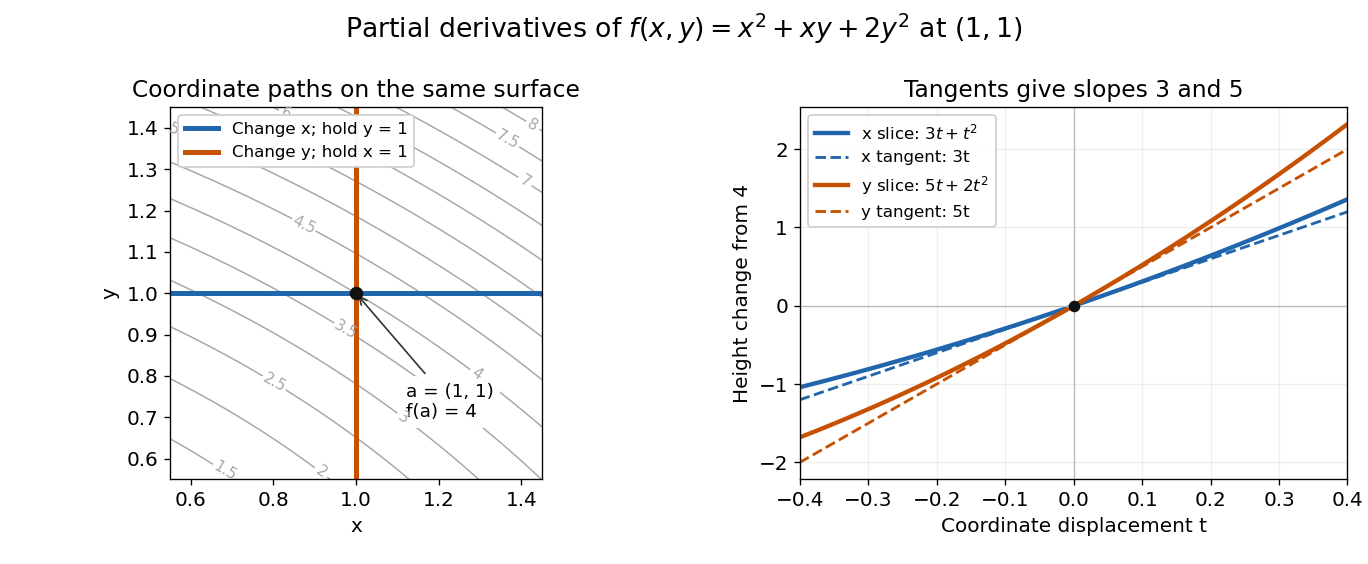
Two coordinate slices through one point give different partial derivatives
. Original contour plot of , with the point and coordinate paths. The right panel compares the exact slice height changes and with their tangent line predictions and . Both slices pass through height . Details.For a function of variables, varies only its th coordinate: it is the same difference quotient along , the th standard basis vector. This gives a practical sensitivity analysis: one can compare how a mathematical model responds to changes in its individual inputs, provided the chosen system of units and the quantities held fixed are stated. Comparing the numerical sizes of two partial derivatives in different units does not by itself identify a physically preferable input.
Existence of the partial derivatives at one point is weaker than differentiability. The example under partial derivatives do not imply continuity shows how both coordinate tests can miss a bad diagonal approach. When the first partial derivatives are continuous in a neighborhood, they do give differentiability there, allowing the total differential to combine all small input changes.
Define away from the origin and zero at the origin. Both partial derivatives exist everywhere and are zero at the origin, yet along the function is , so it is not continuous there. Coordinate-axis derivative tests do not control all neighboring directions.
A mixed partial derivative takes partial derivatives in different variables, for example . If both second partial derivatives are continuous in a neighbourhood, their order can be interchanged: . The chain rule transforms mixed partial derivatives under a linear change of variables by composing the corresponding first-order differential operators.
For away from the origin and zero at the origin, proves Fréchet differentiability with zero derivative. Yet and , giving the displayed unequal mixed partial derivatives. They exist but are not continuous at the origin, so Clairaut's theorem does not apply.
When the second partial derivatives are continuous in a neighborhood, the order of the mixed partial derivatives can be interchanged. Expressing a rectangular finite difference as either iterated integral by the fundamental theorem of calculus and shrinking the rectangle proves the equality. Mere existence of both derivatives does not imply this symmetry.
A time derivative is the partial derivative of an evolving field with respect to time while holding its spatial coordinates fixed. For a quantity depending only on time, it is an ordinary derivative.
The directional derivative tests a function along a chosen straight line, including lines that follow neither coordinate axis. For a fixed vector and a point in an open subset of , defineif the limit exists. With a unit vector , the parameter measures signed distance in the input Euclidean space, so the directional derivative is change per unit distance. For a general , it is change per unit parameter; the norm of also sets the rate of travel.[ref]
4.6 Directional Derivatives and the Gradient. Calculus Volume 3, §4.6, definition (4.36), unit-direction convention
For a differentiable real-valued function, the multivariable chain rule givesThus one gradient predicts the local response in every direction. This formula requires differentiability, rather than merely separate partial derivatives.[ref]
Return to at . Its gradient is . In the unit direction ,One can check this without invoking the gradient formula: substitution givesThe difference quotient is , whose limit is . This calculation separates the exact change along a finite path from its first-order rate at the starting point.
Changing the travel speed changes the parameter rate. Taking gives , because the input travels five distance units per parameter unit. For a differentiable function, for any real : negative reverses the orientation as well as scaling the rate. Normalizing before comparing different slopes avoids confusing direction with speed.
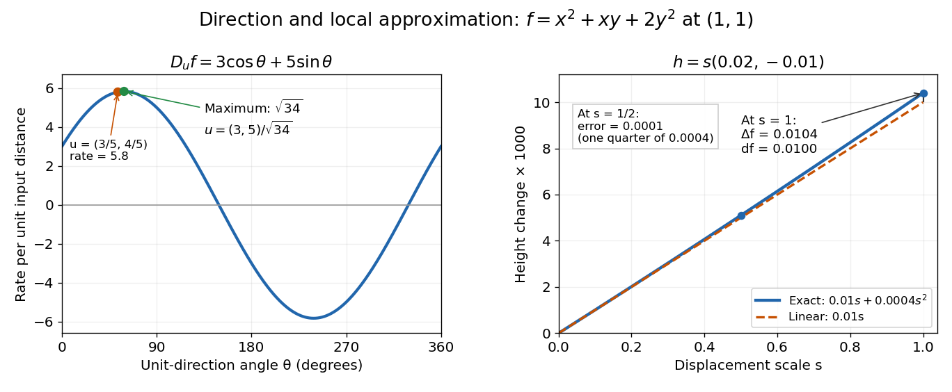
The Cauchy-Schwarz inequality bounds the rate in any unit direction by . Here the largest rate is , attained in the direction ; the chosen gives the slightly smaller rate . The perpendicular unit direction gives zero. That means no first-order height change, rather than no change at all: along this direction the example has .
This is useful for following a height or temperature scalar field, choosing a local search direction in mathematical optimization, and distinguishing a coordinate sensitivity from a response along an actual path. For a curved path, derivative along a curve uses its instantaneous tangent vector. Even existence of all directional derivatives does not guarantee one common linear approximation; directional derivatives do not imply differentiability gives a concrete counterexample.
A functional on a Banach space is Gâteaux differentiable at when the directional limits exist and form a bounded linear functional of . Fréchet differentiability is stronger, requiring a remainder uniformly small compared with the norm of the increment. A quadratic norm bound on the Taylor remainder gives the stronger property directly. Mere existence of unrelated directional limits would not establish linear differentiability.
For , starting at radius and moving radially outward through distance changes the function by . Solving yields the displayed exact distance. Its small-increment limit is , which is the initial directional derivative estimate. That linear estimate is not an exact equality for a specified finite change.
Away from the origin, the radial derivative is the directional derivative along the outward radial unit vector. For a Sobolev space function it is the same scalar product with the weak gradient, defined almost everywhere. On an annulus, it has no singular direction at the origin.
Define away from the origin and zero at the origin. Every directional derivative exists. Along a unit vector , the derivative at the origin is , which is not linear in . Thus these directional derivatives cannot be the restrictions of one Fréchet derivative, and the function is not Fréchet differentiable at that point.
For a locally Lipschitz function that is convex near , increasing secant slopes have a finite right limit. Positive rescaling of gives positive homogeneity in . The convexity bound gives subadditivity after subtracting , dividing by and taking the limit. Thus is a finite sublinear functional, although it need not be a linear functional.
In Cartesian coordinates on Euclidean space, the gradient of a scalar-valued differentiable function is the vector of its first partial derivatives. It converts a scalar field, such as temperature or a height, into a vector field describing its local change.
For a unit vector , the directional derivative is . The Cauchy-Schwarz inequality gives . At a point where , the greatest increase per unit distance occurs along , while the opposite direction gives the greatest decrease. These are first-order statements at the current point; they do not predict how the function behaves far along a straight path.
For at , . Moving in the direction gives rate and moving in the direction gives rate , but the steepest direction is , withThe direction has rate zero and is tangent to the level curve through that point. More generally, differentiating along a regular level curve gives , so the gradient is its normal vector.
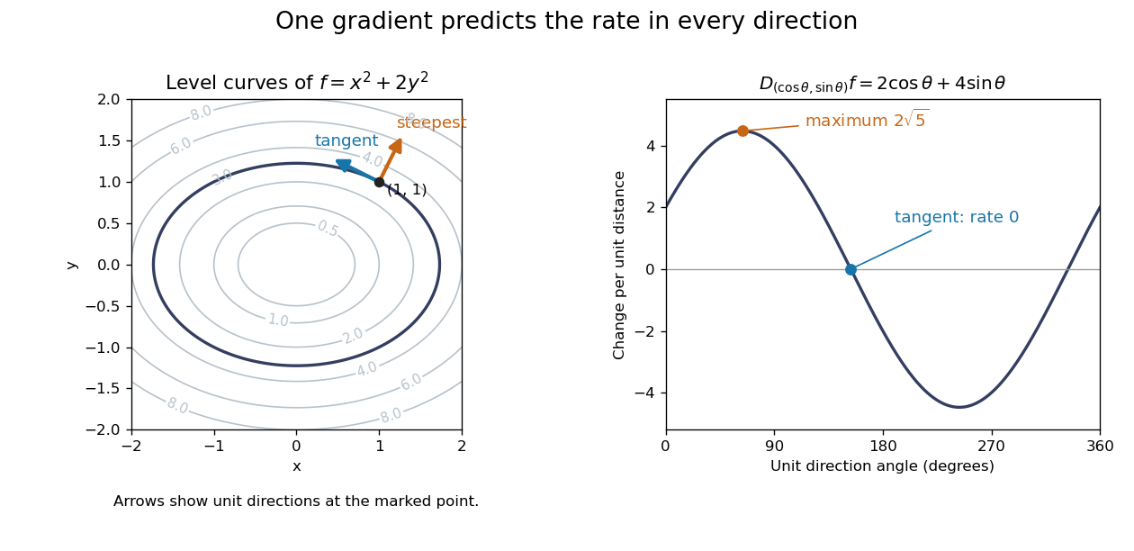
A gradient is normal to level curves and determines the directional derivative for every unit direction
. Details. This is useful when navigating a measured scalar field or applying gradient descent: one collection of partial derivatives predicts every infinitesimal directional change. The derivative assumes a differentiable function, not merely the existence of all directional derivatives. [ref]
4.6 Directional Derivatives and the Gradient. Calculus Volume 3 by Gilbert Strang and others; OpenStax: Directional derivatives and the gradient
.For a differentiable real-valued functional on a real Hilbert space , its functional gradient satisfies for every . A bounded linear derivative has a unique such representative by the Riesz representation theorem. The inner product matters: a formal variational derivative need not equal the functional gradient in another Hilbert space. For in a Reproducing kernel Hilbert space, the reproducing property gives . Substitution in the defining inner product proves this formula directly.
For , the multivariable chain rule givesIndeed, . Thus the gradient points radially outward when , inward when it is negative, and vanishes when it is zero.
At the origin the displayed quotient does not apply. If has a finite right derivative at zero, the radial function is differentiable there exactly when , in which case its gradient is zero. Necessity follows by comparing opposite directional difference quotients: their linear parts cannot both equal a common nonzero radial slope. Sufficiency follows from , the definition of differentiability with zero linear part.
For differentiable vector fields, expand the cross products using the contraction of two Levi-Civita symbols. The directional-derivative terms cancel the corresponding terms in the two cross products, leaving . This proves the displayed gradient identity by the product rule.
A gradient field is a vector field of the form for a scalar potential . Its curl vanishes wherever the required second derivatives commute.
The total differential is the linear map that combines the first-order responses to simultaneous changes in all coordinates. For a differentiable real-valued function at , it can be writtenHere is an input vector; denotes the coordinate linear functional . The coordinate formula and the Fréchet derivative describe the same linear map. The defining approximation isThe little o notation says the remaining approximation error becomes small relative to the input norm, across every direction of approach.[ref]
4.4 Tangent Planes and Linear Approximations. Calculus Volume 3, §4.4, differentiability definition (4.26) and total differential (4.27)
For at , . A simultaneous change gives the linear approximationThe exact algebra isConsequently the exact change is , and the approximation error is . If both input changes are halved, the linear prediction becomes and the error becomes : the first-order response halves, while the quadratic error falls by a factor of four. The right panel under directional derivative displays this comparison as the displacement is scaled.
For a quick check of differentiability, givesDividing by makes this bound tend to zero. The same calculation proves that the tangent plane to the graph of a function at is . It approximates the entire local surface, rather than only two coordinate slices.
The total differential is useful for estimating the combined effect of small input changes without reevaluating a complicated function. For example, if and , then . The exact remainder bound from the displayed polynomial is at most , so this example has throughout that input rectangle. These are deterministic bounds; a variance calculation additionally needs a joint probability distribution and its covariances. A first-order estimate is also local: large changes require control of the remainder, not merely knowledge of the partial derivatives at one point.



