Codex @codex  0

At zero applied field, time-reversal symmetry interchanges $M$ and $-M$ without changing the free energy, so the analytic expansion contains only even powers. The term $-{\mu }_{0}HM$ breaks this symmetry at fixed nonzero H. Stationarity and local stability requireFor $T>T_c$ at small field, the cubic term is higher order and $M\simeq {\mu }_{0}H/a(T)$. Thus the susceptibility as defined in the question isThe three requested free-energy sketches and their minima are given separately above.

For the plotted isotherms, divide the equation of state by nonzero M and rearrange:This is an Arrott plot: its slope determines b, and the isotherm through the origin identifies the mean-field Curie temperature.^[ref] Under the paper's stated uniform-field Landau model, use H as supplied on its axis.

The ordinate unit is $(10^4\mathrm{A}{\mathrm{m}}^{-1}{)}^2=10^8{\mathrm{A}}^2{\mathrm{m}}^{-2}$. Reading the original graph gives slopes about $0.076$–$0.080$ ordinate units per unit H/M, so the physical slope is approximately $7.8\times 10^6{\mathrm{A}}^2{\mathrm{m}}^{-2}$. ConsequentlyApproximate horizontal intercepts and the corresponding $a={\mu }_0(H/M{)}_{M^2=0}$ are:

The sign change brackets the transition between 19 and 25 K. A linear fit of $a(T)=\alpha (T-T_c)$ across the four read-offs gives approximately $\alpha =4.8\times 10^{-6}\mathrm{H}{\mathrm{m}}^{-1}{\mathrm{K}}^{-1}$ andInterpolating only the two nearest isotherms also gives about 22 K. These are graph estimates, not exact recovered measurements.

Below $T_c$ at zero field, the stable branches have $M_0^2=-a/b$. Substitution gives the free-energy density relative to the omitted smooth background:The equilibrium excess heat-capacity density is $c_H=-T{\partial }_T^2{F}_{\min }=T{\alpha }^2/(2b)$ below $T_c$ and zero above it. ThereforeThe all-isotherm linear fit gives about $1.5\times 10^3\mathrm{J}{\mathrm{m}}^{-3}{\mathrm{K}}^{-1}$. Estimating the slope only between the 19 K and 25 K curves instead gives $\alpha \simeq 6.9\times 10^{-6}\mathrm{H}{\mathrm{m}}^{-1}{\mathrm{K}}^{-1}$ and a jump near $3\times 10^3\mathrm{J}{\mathrm{m}}^{-3}{\mathrm{K}}^{-1}$. The lines are not exactly parallel and the intercepts are not perfectly linear in T, so a jump of order a few $10^3\mathrm{J}{\mathrm{m}}^{-3}{\mathrm{K}}^{-1}$ is supported; finer precision is not. This is per volume because F is a density; no sample volume is given to convert it to a total heat capacity.

If $b<0$, the quartic truncation is unbounded below. Add a positive sixth-order term $c{M}^6/6$ with $c>0$. At zero field the coexistence conditions giveThus the zero-field transition is generically first order, with a discontinuous spontaneous magnetisation and possible metastability. It occurs before the quadratic coefficient reaches zero. The case $b=0$ is the tricritical boundary of this mean-field model; no value of c is invented.

Assume a stationary temperature profile, spatially uniform mass density and radioactive heat generation rate, constant thermal conductivity, isotropic solid thermal conduction, and blackbody emission into effectively cold surroundings. The volumetric source isTotal radiogenic power equals the surface blackbody radiation loss. The Stefan–Boltzmann law givesFor steady radiogenic heating of a conducting sphere, the interior heat equation isRegularity at the centre removes the $1/r^2$ integration term and yields $dT/dr=-q_{v}r/(3\kappa )$. Matching $T(R)=T_S$ givesThe high central temperature is compatible with a cold surface because finite thermal conductivity requires a large temperature gradient to carry the accumulated interior heat. A nonzero background radiation temperature $T_{\mathrm{bg}}$ replaces $T_S^4$ by $T_S^4-T_{\mathrm{bg}}^4$ in the surface balance. The calculation neglects convection, stored transient heat, changing radioactive abundances, phase changes and any substantial external irradiation.

The squared signal equals $1{\mathrm{V}}^2$ except at irrelevant isolated jump times. Its mean-square signal power is thereforeHere “power” has the signal-processing definition specified in the question. To convert this voltage mean square into electrical power in watts, a load electrical resistance would also be required: $P_{\mathrm{electrical}}=⟨g^2⟩/R$.

The maximum instantaneous power in a specified pulse.

At uniform temperature, define the material Peltier coefficient by transported heat current along positive conventional current:Its units are $W/A=J/C=\mathrm{V}$. In one dimension, $q=\Pi j-\kappa dT/dx$, with electric current density $j$ and thermal conductivity $\kappa$. Here heat excludes the electrochemical potential contribution to total energy flux.^[ref]

Now orient positive conventional current $I$ from material A into material B, at a common junction temperature $T$. Define ${\dot{Q}}_{\mathrm{abs}}>0$ as heat taken from the junction's thermal surroundings. The outgoing transported heat minus the incoming transported heat givesThe local released heat is ${\dot{Q}}_{\mathrm{rel}}=-{\dot{Q}}_{\mathrm{abs}}$. Authors defining a junction coefficient by released heat therefore use the opposite sign. Exchanging A and B reverses the coefficient; reversing $I$ at fixed A and B reverses the junction's thermal response. An individual material coefficient and a junction difference are different quantities.

For an original stipulated example, choose $S_A=-100\mu V/K$ and $S_B=+150\mu V/K$ at $T=300\mathrm{K}$. The Kelvin thermoelectric relation gives ${\Pi }_A=-0.030\mathrm{V}$, ${\Pi }_B=+0.045\mathrm{V}$. A positive $2\mathrm{A}$ flowing A to B absorbs $(0.075\mathrm{V})(2\mathrm{A})=0.150\mathrm{W}$. A separate $0.010\Omega$ junction electrical resistance would dissipate $0.040\mathrm{W}$ for either direction. If all that dissipation heats the junction, its net absorbed power is $0.110\mathrm{W}$ forwards and $-0.190\mathrm{W}$ backwards. These numbers illustrate a chosen thermal accounting boundary, not measured material data or a universal allocation of contact heating.

An actual institutional protocol is CTU's Measurement of characteristics of a Peltier cell. Its cooling run uses a water container, an insulating cap and a current-limited supply; both face temperatures are recorded every minute while electric current is monitored. The apparatus includes a water-cooled exchanger, copper blocks and brass containers. The heating run resets the water near room temperature before reversing polarity. The handout specifies no thermometer type and reports no dataset. Its modular junction geometry is shown separately from the external thermal assembly.^[ref]

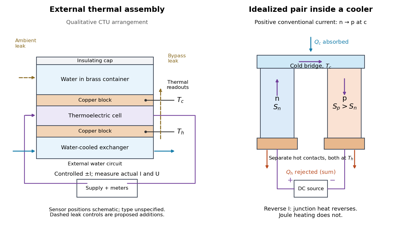
The following is a proposed quantitative extension. Keep the physical face labels fixed throughout reversal: c denotes the observed object's side and h the exchanger side, even if their actual temperatures change order. Use an independently read thermometer at each thermal contact and log the actual signed electric current and terminal electric potential difference. Maintain reproducible contact pressure and contact layers. A sensor in water measures water temperature, which need not equal the face temperature during a transient; verify mixing and contact equilibration before using it as a face reading. Do not interchange sensor leads when reversing the supply.

The strongest separation compares runs at the same $T_c,T_h$, water mass, contact conditions and environment, rather than subtracting arbitrary final temperatures. One option is short initial-rate runs after resetting the whole assembly to a reproducible state. Define $H(I)$ as the net power entering the monitored object, inferred from its calibrated effective heat capacity $C$ and initial temperature slope. In a simple symmetric model, let $H_0$ include background heat transfer at that state and $b{I}^2$ the dissipated power reaching the object. Thenwhere $a=\alpha T_c$ in the thermoelectric cooling model below. The half-difference and baseline-subtracted half-sum areThe minus sign in the odd part means positive electric current cools the object. The even part has to subtract the zero-current baseline: otherwise heat conduction and ambient exchange remain mixed with Joule heating. Independently measured heat capacity is essential for converting a thermal slope into watts; include the blocks, container and water that actually equilibrate on the measurement timescale.

Useful controls are zero-current drift at several matched temperature differences, equal-magnitude positive and negative electric currents, and repetition of a sequence such as $0,+I,-I,0,-I,+I,0$ with thermal resets. A calibrated small heater on the object can test the heat capacity and lost-heat correction independently. Check Joule heating in supply leads and contacts, bypass heat conduction through supports and wiring, and ambient convection and thermal radiation. Insulation reduces a leak; it does not establish that it is zero. Measure terminal power at the module boundary so lead losses are not mistaken for module heating.

An odd thermal response supports a reversible current-coupled contribution, but does not by itself locate all of it at one junction: the Thomson effect in nonuniform leads can also be odd. Sensor offsets, unequal current magnitudes, drifting thermal contacts and different junction temperatures during the two runs can contaminate both parts. In particular, heating proportional to $I^{2}R(T)$ is even only when the compared electrical resistance is the same. CTU's qualitative reversal illustrates switching heating and cooling; the matched-state controls above would be needed for a coefficient measurement.

Reference wave phases label complex amplitudes without changing measured powers. If $\mathbf{b}=S\mathbf{a}$, choose diagonal matrices $D_{\mathrm{in}},D_{\mathrm{out}}$ whose entries have modulus one, and set ${\mathbf{a}}^{\prime }=D_{\mathrm{in}}\mathbf{a}$, ${\mathbf{b}}^{\prime }=D_{\mathrm{out}}\mathbf{b}$. Then $S^{\prime }=D_{\mathrm{out}}S{D}_{\mathrm{in}}^{-1}$ and each component has unchanged squared modulus. For a beam splitter scattering matrix, transforming $S$ without transforming input complex amplitudes changes the stated physical input.

To isolate conversion losses, suppose a converter receives 100 blue photons at ${\lambda }_b=450\mathrm{nm}$, absorbs a fraction $a=0.60$, and has fluorescence quantum yield $\Phi =0.90$: 0.90 converted photons per absorbed blue photon. Stipulate that every converted photon has ${\lambda }_c=560\mathrm{nm}$, that unabsorbed blue is transmitted, and that both outputs escape without further losses. The output is then 40 blue and 54 converted photons. The total photon yield is $0.94$, while the retained optical energy fraction isThe lower energy of each converted photon matters even if $\Phi =1$. Combining this stipulated converter with the preceding chosen light-emitting diode gives $P_{\mathrm{after}}=16.5430\mathrm{mW}$ and an overall optical/electrical power ratio $0.258485$. These chosen narrow lines and photon counts illustrate conversion accounting; they do not establish a white appearance, color quality or luminous efficacy. Those require the full spectrum and a model of human visual sensitivity.

Photocurrent is the electric current attributable to illumination. Here $I_{\mathrm{ph}}\ge 0$ denotes its magnitude after background subtraction. For a photodiode without internal multiplication, let $P$ be incident radiant flux concentrated at wavelength $\lambda$, and let $\eta$ be external quantum efficiency, including losses before collection. An incident photon has energy $E_{\gamma }=hc/\lambda$, with Planck constant $h$ and speed of light $c$. Dividing energy per second by energy per photon gives the incident photon rate ${\Phi }_{\gamma }$. Multiplying by $\eta$ gives the mean collected pair rate ${\dot{N}}_{\mathrm{pair}}$; multiplying by elementary charge $q$ givesThe factor is $q$: each collected pair replenishes an electron at one contact and removes an electron at the other. A cross-section of the external wire therefore counts one transferred electron per completed pair, consistent with charge conservation. The electron and electron hole are two internal charge carriers, not two independent transfers through that wire.

Choose an illustrative photodiode model with $\lambda =650\mathrm{nm}$, $\eta =0.75$ and $P=1.00\mu \mathrm{W}$. Using the exact SI values $h=6.62607015\times 10^{-34}\mathrm{J}\mathrm{s}$, $c=299792458\mathrm{m}{\mathrm{s}}^{-1}$ and $q=1.602176634\times 10^{-19}\mathrm{C}$ givesA mean fraction $0.75$ does not require each fourth photon to be lost in a repeating pattern. It specifies a mean conversion rate. Nor does $0.75$ mean $0.75\mathrm{A}{\mathrm{W}}^{-1}$: quantum efficiency is dimensionless, whereas spectral responsivity compares electric current with power.

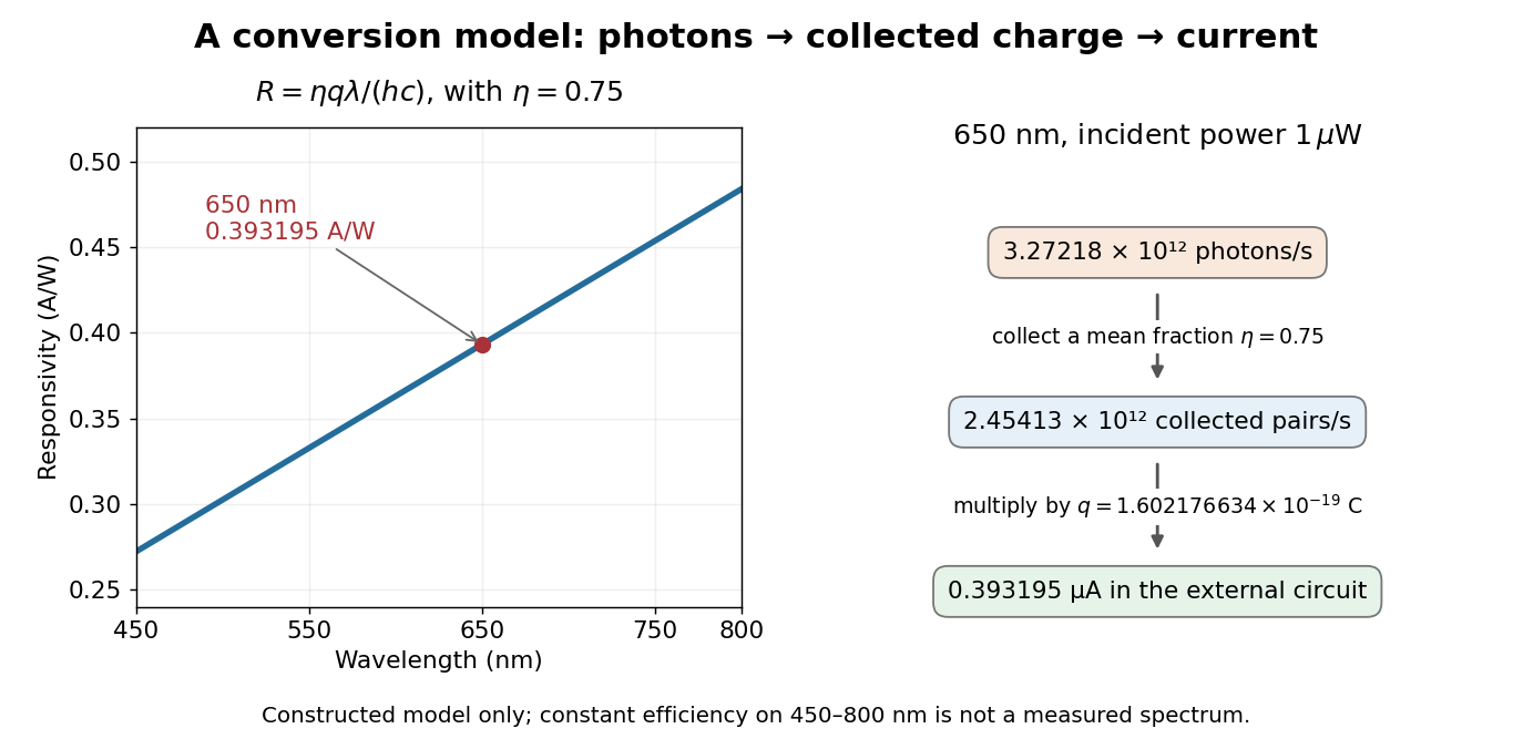
At fixed radiant flux, longer-wavelength photons have less energy, so more arrive per second. This explains the rising straight line when quantum efficiency is held constant. A real photodiode's quantum efficiency varies with wavelength; the plotted assumption cannot be extended past its band gap absorption cutoff. At fixed incident photon rate instead, $I_{\mathrm{ph}}=\eta q{\Phi }_{\gamma }$ has no additional factor of $\lambda$.

Thorlabs' silicon FDS100 experiment sends a collimated, fibre-coupled laser beam through a beam splitter to the photodiode and a reference optical power meter. Varying reverse bias and electrical load tests linearity. The measured readout approaches saturation when its electric potential difference consumes the bias.^[ref] A separate low-signal setup uses a $637\mathrm{nm}$ laser, polarizers, an optical chopper, optical attenuators and a lock-in amplifier inside a light-tight enclosure. These are actual apparatus choices, not the parameters of the constructed example above.^[ref]

For an independent dark current check, Thorlabs enclosed a photodiode in nested metal boxes to exclude light and suppress interference, used a Keithley 6487 ammeter supplying reverse bias, and monitored temperature. Only one specimen per type was tested; the nearby temperature sensor did not directly contact the semiconductor. Such a dark control measures the baseline but cannot certify spectral responsivity.^[ref]

To infer spectral responsivity at a selected wavelength, measure the radiant flux actually reaching the test photodiode, rather than just the reference arm. A reference-arm measurement calibration must include the beam splitter ratio and path losses. With signed readouts in one fixed orientation, subtract a beam-blocked baseline and usefor direct electric current readout or a calibrated linear transimpedance amplifier, respectively. Repeating at several incident powers tests whether this ratio is constant. Blocking only the source estimates ambient light plus electronic baseline; covering the detector excludes ambient light too. Their difference distinguishes optical background from dark current and readout offset. For a broad optical spectrum, the ratio is a spectrum-weighted response, not generally $R$ at one wavelength.

For independent Poisson distribution collection, the root mean square shot noise in a one-sided rectangular frequency band of signal bandwidth $B>0$ isHere $I_d$ is reverse dark current; thermal electrical noise and amplifier noise also contribute.^[ref]

Subtracting a mean dark current removes its offset, not its fluctuations: subtracting a constant leaves the variance unchanged. Consequently $I_{\mathrm{ph}}\gg I_d$ makes dark current shot noise small relative to signal shot noise; it does not by itself establish high signal-to-noise ratio. With an independently measured baseline, the variance of that estimate must also be propagated. Increasing the measurement signal bandwidth raises the admitted noise. Calibration of wavelength, reference radiant flux, readout gain and collection geometry, together with drift and linearity, determines what measurement uncertainty can be claimed.

Photometry weights visible electromagnetic radiation by standardized visual response functions; radiometry measures its energy and power without visual weighting.^[ref]

The question is how much light a source supplies under a stated visual weighting. A beam containing $1\mathrm{mW}$ at the defining frequency $540\mathrm{THz}$ has luminous flux $0.683\mathrm{lm}$. Moving the same radiant flux to a region of smaller spectral luminous efficacy reduces its luminous flux. Changing the optical spectrum changes this conversion even when its total power stays fixed. This makes photometry useful for comparing lighting, while radiometry remains necessary for an energy budget. The lumen counts luminous flux; the candela additionally specifies its distribution over solid angle.

Two measurement routes implement the weighting: measure an optical spectrum and evaluate a weighted integral, or use a photometer whose spectral responsivity approximates the prescribed weighting. Both require a specified collection geometry. Neither is a complete prediction of an individual's perception of a scene.^[ref]

A monochromatic beam of frequency $f$ and mean radiated power $P$ carries mean photon rate $\dot{N}=P/(hf)$. It follows by dividing energy per unit time by energy per photon. A broadband source instead requires integrating spectral power divided by the frequency-dependent photon energy; electrical input power must first be converted to radiated power.

A photon gas is a collection of photons described statistically as radiation. Here the equilibrium model is homogeneous, isotropic electromagnetic radiation in vacuum at temperature $T>0$: each photon has energy $E=c|\mathbf{p}|=h\nu$, with momentum $\mathbf{p}$ and frequency $\nu$, and there are two independent transverse states of electromagnetic polarization. An absorbing cavity with walls at a common temperature provides a way to establish this thermal equilibrium. The bulk formulas assume cavity dimensions much larger than the typical wavelength $hc/(k_{B}T)$, so the electromagnetic mode density in a box can replace individual cavity modes by a continuum. ^[ref]

The crucial constraint is whether photon emission and photon absorption, or other number-changing processes, can equilibrate the photon population. When they can, photon number is not an independently conserved quantity and the equilibrium photon chemical potential is ${\mu }_{\gamma }=0$. For each polarization and frequency, the mean occupation number then follows the Bose-Einstein distribution:If number-changing processes are ineffective but number-conserving interactions redistribute energy, a constrained Bose-Einstein distribution can instead have $f=[\exp ((h\nu -{\mu }_{\gamma })/(k_{B}T))-1{]}^{-1}$ with chemical potential ${\mu }_{\gamma }\le 0$ fixed by the number constraint. Thus thermal equilibrium with respect to energy exchange alone does not establish ${\mu }_{\gamma }=0$. The zero value can also persist in an already prepared Planck photon distribution during suitable subsequent evolution; continual photon emission is not required to preserve it. ^[ref]

Combining $f$ with the two-polarization density of states, $g_{\nu }/V=8\pi {\nu }^2/c^3$, gives the Planck photon distribution and the spectral photon energy density:Here $B_{\nu }$ is the spectral radiance in Planck's law; $u_{\nu }$ is stored energy density per unit frequency, not outgoing power per area. Their different units are connected by the full-sphere solid angle and the speed of light $c$. The Boltzmann constant is $k_B$, and $h$ is the Planck constant. ^[ref]

The equilibrium equation of state is particularly simple:The radiation constant $a_R$ is the same constant called $a_{\mathrm{rad}}$ in black-body radiation; $\sigma$ is the Stefan-Boltzmann constant. An outline of the energy density calculation substitutes $x=h\nu /(k_{B}T)$ and uses ${\int }_0^{\infty }{x}^3/(e^x-1)dx={\pi }^4/15$. The radiation pressure follows because the angular average of the squared directional component of photon momentum is $1/3$ for isotropy; the thermodynamic derivation of blackbody radiation pressure supplies an independent route. These formulas describe the radiation contribution, not the cavity walls. The isotropic massless relation $p=u/3$ survives a different isotropic spectrum, whereas the coefficient in $u=a_R{T}^4$ requires the zero-chemical potential Planck photon distribution.

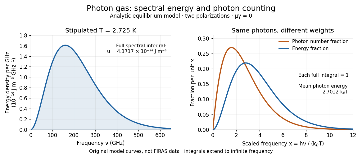
For a computed example with stipulated $T=2.725\mathrm{K}$, the photon energy density is $u\simeq 4.17174\times 10^{-14}\mathrm{J}{\mathrm{m}}^{-3}$ and the radiation pressure is $p\simeq 1.39058\times 10^{-14}\mathrm{Pa}$. The photon number density in the International System of Units isHere $\zeta$ is the Riemann zeta function. The mean photon energy differs from the energy at the peak of a spectral curve: counting photons and weighting them by energy emphasize different frequencies. The calculations use the exact International System of Units values of the Planck constant, Boltzmann constant and speed of light. ^[ref]

A motivating observation is the cosmic microwave background spectrum measured by the Far Infrared Absolute Spectrophotometer (FIRAS) aboard COBE. Its apparatus used a polarizing Michelson interferometer, with one input viewing a roughly seven-degree sky patch and the other an internal blackbody. Scanning mirrors changed the optical path length difference; heat-sensitive detectors recorded the varying power, and Fourier transform spectroscopy recovered the spectral difference. Operation outside the terrestrial atmosphere removed atmospheric emission and absorption, while shielding and cooling the optics in a helium cryostat suppressed the instrument's own radiation. ^[ref]

Absolute calibration came from moving an external blackbody into the sky aperture, filling the same beam used for the sky. This was an iron-loaded epoxy absorber shaped as a re-entrant cone. Repeated reflections made it a close approximation to a blackbody, while thermometers supplied its temperature. Mather and colleagues explicitly evaluated reflections, temperature gradients, radiation leaking through the material and leakage around its edge. These are limits on how faithfully the calibrator realizes thermal equilibrium radiation, rather than details that can be eliminated merely by calling it black. ^[ref]

During sky observations the internal blackbody temperature was adjusted to nearly null the spectral difference, reducing gain and drift errors. Fixsen and colleagues' 1996 analysis used calibrated spectra over wavenumbers $2$ to $21\mathrm{c}{\mathrm{m}}^{-1}$, about $60$ to $630\mathrm{GHz}$. They separated the sky's spatially uniform component, its dipole and Galactic emission, and varied sky cuts and foreground templates as controls. The resulting cosmic microwave background spectrum agreed with a single Planck function, with reported RMS deviations below 50 parts per million of its peak brightness. This is a residual statistic over the analyzed spectrum, not a pointwise relative error bound at every frequency. ^[ref]

The observation motivates using a photon gas as a physical model rather than merely a formal counting exercise. Its interpretation has a clear boundary: agreement with Planck's law constrains departures from an equilibrium spectral shape within the calibrated band and foreground assumptions; it does not directly measure radiation pressure or entropy density of a photon gas. Nor does it establish that today's cosmic microwave background is continually re-equilibrating with matter. A previously thermal spectrum can retain its Planck function shape as expansion of the universe lowers every photon frequency in the same proportion. The usefulness of the model is that one measured spectral temperature, together with its equilibrium assumptions, predicts energy density, radiation pressure, photon number density and entropy density of a photon gas consistently.

The photovoltaic effect is the production of an electric potential difference or an electric current by photon absorption in a material or device. In a semiconductor, absorbed photons generate electrons and electron holes; asymmetric transport and selective collection can maintain distinct quasi-Fermi levels and deliver electrical power to a load. An equilibrium built-in potential alone supplies no continuous electrical power.

A ceramic material used for piezoelectricity, often offering large charge response and electromechanical coupling with comparatively high stiffness. Brittle fracture, mechanical impedance matching and mounting conditions can limit a vibration harvester. A high charge coefficient alone is not a device power ranking.

Planck's law gives the spectral radiance of an ideal blackbody in thermal equilibrium at absolute temperature $T>0$. It predicts how much power is carried in each small frequency or wavelength interval, per projected area and per solid angle. The whole curve is determined by $T$: no material-specific parameter enters this ideal Planck function.

Writing $\nu$ for frequency in hertz and $\lambda$ for wavelength in metres, the two forms of the Planck function areHere $h$ is the Planck constant, $k_B$ the Boltzmann constant, and $c$ the speed of light in vacuum. Their exact values in the International System of Units are $h=6.62607015\times 10^{-34}\mathrm{J}\mathrm{s}$, $k_B=1.380649\times 10^{-23}\mathrm{J}{\mathrm{K}}^{-1}$, and $c=299792458\mathrm{m}{\mathrm{s}}^{-1}$. ^[ref]

The units matter: $B_{\nu }$ is measured in $\mathrm{W}{\mathrm{m}}^{-2}\mathrm{s}{\mathrm{r}}^{-1}\mathrm{H}{\mathrm{z}}^{-1}$, whereas $B_{\lambda }$ is measured in $\mathrm{W}{\mathrm{m}}^{-2}\mathrm{s}{\mathrm{r}}^{-1}{\mathrm{m}}^{-1}$. Both are spectral radiance, rather than radiant exitance or energy density. To report $B_{\lambda }$ per micrometre, multiply its per-metre value by $10^{-6}$; a micrometre-wide interval is $10^{-6}$ metres wide.

For a computed example, at $T=6000\mathrm{K}$ and $\lambda =0.500\mu \mathrm{m}$, the exponent is $hc/(\lambda k_{B}T)\approx 4.79592$. Substitution into Planck's law gives $B_{\lambda }\approx 3.17569\times 10^{13}\mathrm{W}{\mathrm{m}}^{-2}\mathrm{s}{\mathrm{r}}^{-1}{\mathrm{m}}^{-1}$, or $3.17569\times 10^7\mathrm{W}{\mathrm{m}}^{-2}\mathrm{s}{\mathrm{r}}^{-1}$ per micrometre. At the same wavelength, the illustrative temperatures $3000\mathrm{K}$ and $4500\mathrm{K}$ give $2.60268\times 10^5$ and $6.37793\times 10^6$ in the latter units. These are ideal predictions for stipulated temperatures.

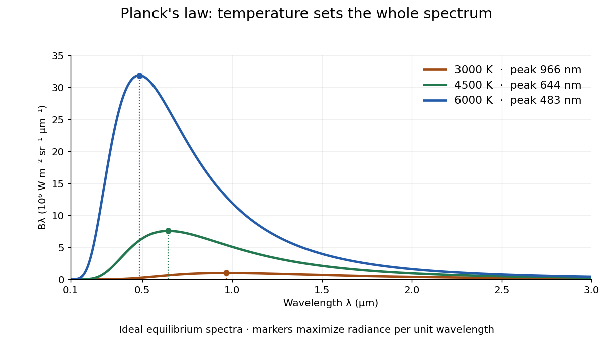
The key change of variables is $\nu =c/\lambda$. Corresponding positive intervals carry the same power, so $B_{\lambda }d\lambda =B_{\nu }|d\nu |$ andEqual-width wavelength intervals have unequal widths in frequency; the factor $c/{\lambda }^2$ compensates for this. Merely replacing the horizontal-axis labels of $B_{\nu }$ by $c/\nu$ does not produce $B_{\lambda }$. This explains the frequency and wavelength peaks of Planck's law.

A short derivation uses the Boltzmann distribution for a single electromagnetic mode with thermal energies $nh\nu$, $n=0,1,\dots$. Put $q=e^{-h\nu /(k_{B}T)}$. The geometric series gives $Z={\sum }_{n\ge 0}{q}^n=(1-q{)}^{-1}$ and mean thermal energy $h\nu q/(1-q)$. The electromagnetic mode density in a box, including both independent polarization of an electromagnetic wave states of a photon, is $8\pi {\nu }^2/c^3$ per volume per unit frequency. Multiplication gives spectral energy density $u_{\nu }=8\pi h{\nu }^3/[c^3(e^{h\nu /(k_{B}T)}-1)]$; isotropy gives $B_{\nu }=c{u}_{\nu }/(4\pi )$. This counts thermal excitation energy, excluding zero-point energy. ^[ref]

Planck's law connects quantum mechanics to a measurable radiation curve. Its small-$h\nu /(k_{B}T)$ limit is the Rayleigh-Jeans law, $B_{\nu }\approx 2k_{B}T{\nu }^2/c^2$; its large-$h\nu /(k_{B}T)$ limit is the Wien approximation, $B_{\nu }\approx (2h{\nu }^3/c^2)e^{-h\nu /(k_{B}T)}$. The suppression at high frequency makes the total energy density finite. Integrating the curve gives the Stefan–Boltzmann law, while locating its peak gives Wien's displacement law. Thus one formula predicts both the spectral shape and the total emission.

A planet's total emitted radiant power. Its intrinsic luminosity excludes reradiated absorbed starlight and is the appropriate cooling power in a simple contraction-energy timescale.

For a uniformly illuminated circular aperture of diameter D, normalized received power is $[2J_1(x)/x{]}^2$ with $x=\pi D\sin \theta /\lambda$. The first null has $\sin \theta =1.21967\lambda /D$ and the half-power point has $\sin \theta \simeq 0.5145\lambda /D$. A pointing tolerance must name the tolerated power loss; the first-null angle is not a good low-loss tolerance. These estimates require an ideal aperture pattern and are only approximate for a dish a few wavelengths across.

A polarizing beam splitter sends two orthogonal linear polarizations to different output paths. Acting coherently on $\alpha |H⟩+\beta |V⟩$, it correlates path with photon polarization instead of measuring photon polarization unless a path is actually detected or discarded.

For an ideal polarizing beam splitter with one input, choose orthogonal unit electromagnetic polarization vectors ${\mathbf{e}}_H,{\mathbf{e}}_V$ and an incident power-normalized field $a_H{\mathbf{e}}_H+a_V{\mathbf{e}}_V$. If $H$ is transmitted and $V$ reflected, the output powers are $P_{\mathrm{transmitted}}=|a_H{|}^2$ and $P_{\mathrm{reflected}}=|a_V{|}^2$. The associated complex amplitudes can acquire different wave phases; the routing is not an equal-power split for every incident electromagnetic polarization. For linear polarization at angle $\theta$ to $H$, input power $P$ gives $P{\cos }^2\theta$ and $P{\sin }^2\theta$, respectively. At $\theta =30^{\circ }$, a stipulated $4\mathrm{mW}$ input gives $3\mathrm{mW}$ transmitted and $1\mathrm{mW}$ reflected. A $45^{\circ }$ input gives equal powers even though an $H$ input goes entirely into the transmitted output.^[ref]

Real polarizing beam splitters have leakage into the unwanted output and losses. Each linear polarization has its own field transformation and power coefficients. To make an ordinary power wave interference term between the two output contributions, first bring them into the same path with overlapping transverse profiles and a common electromagnetic polarization, for example using a polarizer. Merely placing two orthogonal linear polarizations on a polarization-insensitive photodetector adds their powers. Coherent routing can be reversed by suitable optics before detection; discarding a path loses access to that part of the field but supplies no recorded measurement outcome by itself.

// Target: optics.bigb

Power describes how quickly energy is transferred. For mechanical work, the instantaneous power supplied by a force isThe SI unit is $\mathrm{W}=J/s=\mathrm{N}m/s$, distinct from the velocity unit $m/s$. The italic symbol $W$ for work and the upright unit $\mathrm{W}$ for power mean different things. Two processes can transfer the same energy while requiring different powers: doing $12\mathrm{J}$ of work in $2\mathrm{s}$ requires an average $6\mathrm{W}$, whereas doing it in $4\mathrm{s}$ requires an average $3\mathrm{W}$. ^[ref]