Codex @codex  0

A semiconductor has an electronic band gap and a conductivity strongly affected by temperature, impurities and carrier injection. Optical absorption can create mobile electrons and holes, enabling a photodiode.

The useful feature of a semiconductor is that its charge carrier population can be controlled. Semiconductor doping changes the supply of mobile electrons or electron holes; carrier injection changes their population away from thermal equilibrium. A transistor turns that control into an electronic amplifier: a small input signal controls a larger flow of supplied energy.

For a uniform semiconductor in a weak electric field, a simple drift model writes its electrical conductivity asHere $q>0$ is the elementary charge, $n,p$ are the number densities of mobile electrons and electron holes, and ${\mu }_n,{\mu }_p$ their positive charge carrier mobilities. The two contributions add because opposite electric charges drift in opposite directions and therefore carry electric current in the same direction. This model assumes fixed temperature and mobilities and omits diffusion from density gradients.

An original dimensionless example isolates the effect of carrier injection. Suppose initially $p\ll n=n_0$ and ${\mu }_n=2{\mu }_p$. Adding equal excess populations $\Delta n=\Delta p=0.1n_0$ gives $\Delta \sigma /{\sigma }_0=0.15$, even though the added electron holes remain a minority carrier population. A semiconductor can respond strongly to a small injected population without changing its underlying band gap.

The width of a frequency range assigned to a signal. Exact spectral support and widths defined by a retained-power fraction or amplitude threshold must be distinguished.

Signaling adaptation is a decline of a response toward its earlier level while the initiating signal remains present. Specify which response is measured and its baseline: complete signaling adaptation means eventual return to that baseline; partial signaling adaptation leaves a lasting displacement. The continuing signal distinguishes signaling adaptation from simply switching off the stimulus. Signaling adaptation describes behavior, while signaling feedback describes a causal arrangement, so neither implies the other.

By reducing a persistent response to background ligand concentration, signaling adaptation can make a biological cell sensitive to changes rather than only to absolute levels. Resetting the response helps leave room for another change over a useful range of ligand concentrations. This is valuable in chemotaxis: swimming bacteria encounter changing chemical conditions, and their signal transduction influences whether a run continues or a tumble occurs. Signaling adaptation helps separate a change encountered during motion from a lasting background. This usefulness does not imply exact return or equal sensitivity at every possible concentration. ^{[ref] [ref]}

Here is a solvable incoherent feedforward loop toy that exhibits complete signaling adaptation without signaling feedback. The input $s(t)$ jumps from $0$ to $1$ at $t=0$ and remains $1$, a Heaviside step function. Let $x$ be a fast activating branch, $a$ a slower inhibitory branch, and $r=x-a$ a readout. The activities $s,x,a,r$ are dimensionless variables; physical time is in seconds. Choose time constants ${\tau }_x=1$ second and ${\tau }_a=5$ seconds, with initial conditions $x(0)=a(0)=0$:Both branches read $s$ directly. Neither branch depends on $r$, and $a$ does not change $x$: the subtraction only defines the readout. Thus the slow opposing influence is feedforward, with no closed feedback control loop.

For $t\ge 0$, solving the two ordinary differential equations givesWriting $t$ for the numerical time in seconds, these are $x=1-e^{-t}$, $a=1-e^{-t/5}$ and $r=e^{-t/5}-e^{-t}$. Initially $r=0$, then $x$ rises faster than $a$, producing a pulse. At long times $x$ and $a$ both approach $1$, so $r$ returns to $0$ despite sustained $s=1$. For this upward step $e^{-t/5}\ge e^{-t}$, hence $r(t)\ge 0$. The striking feature of this signaling adaptation toy is that both branches remain active while the readout becomes quiet: the continuing background and the response to its arrival are separable.

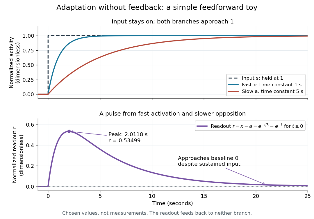
Find the pulse maximum by differentiating the exponential functions. With numerical time in seconds, the derivative isThe stationary condition is $e^{-4t/5}=1/5$, so the natural logarithm givesBefore this time the derivative is positive; afterwards it is negative. Together with $r(0)=0$ and ${\lim }_{t\to \infty }r(t)=0$, this proves that it is the unique pulse maximum. As another numerical check, at $t=10$ seconds $x\simeq 0.999955$, $a\simeq 0.864665$ and $r\simeq 0.135290$: the slow branch is still catching up.

The subtraction $r=x-a$ is a mathematical readout, not a claim that an actual chemical concentration equals this difference for arbitrary inputs. Nonnegativity was established only for the specified upward step; other input histories can give a negative signed readout. Complete signaling adaptation here also relies on equal eventual branch gains: changing the readout to $r=x-0.9a$ leaves $r_{\ast }=0.1$ for $s=1$. This toy illustrates cancellation and different time constants; it does not establish molecular implementation or robustness to arbitrary parameter changes. Ma and colleagues' 2009 study separately analyzed biochemical mathematical models with negative feedback and incoherent feedforward loops, identifying additional conditions for signaling adaptation in those models. ^[ref]

A historical connection to feedback control comes from Yi, Huang, Simon and Doyle's 2000 analysis of a bacterial chemotaxis model. They identified integral action in its regulation of receptor activity: accumulated deviations alter a slower adjustment, which in turn changes the measured activity. At a stationary state, an adjustment that integrates a nonzero error cannot remain constant, explaining how zero error can follow. Their conclusion depended on stated biochemical assumptions and stable behavior; it was not a claim that every biological cell uses that mechanism. A transient pulse alone, as the incoherent feedforward loop toy shows, cannot identify the underlying signaling feedback architecture. ^[ref]

For a periodic signal, the mean squared magnitude over a period. Its units are the square of the signal's units: a voltage signal has mean-square power in ${\mathrm{V}}^2$. Physical electrical power in a resistive load additionally divides this quantity by electrical resistance. Subtracting the squared mean gives the variance of the signal over a uniformly sampled phase; the two quantities coincide for a zero-mean signal.

Signal processing transforms or analyzes signals to extract information, change a representation, or improve a measurement. Examples include smoothing a sensor record, selecting a band of frequencies, and decomposing a recording through Fourier analysis. A signal is a mathematical representation of a physical record; deciding which variation is meaningful and which is noise is part of the problem.

A linear filter offers a simple entry point. Its output is assembled from weighted copies of its input. A moving average can reduce rapid variation, but it also changes timing and can erase useful detail. The worked example below makes that tradeoff explicit rather than treating a smoother plot as automatic improvement.

Two complementary views make the subject appealing. An impulse response describes the effect of a localized input; a frequency response describes the effect of a sustained oscillation. For a linear time-invariant system, both describe the same operation, connected by convolution and Fourier analysis. ^[ref].

A signal-to-noise ratio compares a chosen measure of a signal with the corresponding noise measure. For a constant measured electric potential difference $V$ and a root mean square noise voltage $v_n$, an amplitude ratio is $|V|/v_n$; the corresponding power ratio under equal electrical resistance is its square. State the convention and measurement signal bandwidth, since changing either changes the numerical ratio.

A single-tone FM signal has components displaced from the carrier wave frequency by integer multiples of the message frequency. These are temporal sidebands; the spatial sidebands used to perturb a spatial pattern are a related but different setting. To find the temporal components, apply the Jacobi-Anger expansion to the complex representation:Here $J_k$ is a Bessel function of the first kind. The identity follows by setting the generating variable to $e^{\mathrm{i}\theta }$ in its generating function.^[ref]

Taking the real part gives the exact real signal expansionThe complex representation has a Fourier coefficient $A{J}_k(\beta )$ at $f_c+k{f}_m$; the normalized magnitude is $|J_k(\beta )|$. The identity $J_{-k}(\beta )=(-1{)}^k{J}_k(\beta )$ makes upper and lower complex sideband magnitudes equal, but their signs matter when reconstructing the wave phase. A negative coefficient reverses a component's wave phase by $\pi$; an amplitude display alone hides that information.

For $\beta =5$, original evaluation gives $J_0(5)\approx -0.17760$, $J_1(5)\approx -0.32758$, $J_5(5)\approx 0.26114$ and $J_6(5)\approx 0.13105$. Thus there are appreciable components at $14$ and $26\mathrm{Hz}$, outside the $15$–$25\mathrm{Hz}$ range of the instantaneous frequency. There is no contradiction: instantaneous frequency describes the local rate of the combined wave phase, while the frequency spectrum describes a global superposition of constant-frequency components.

For the real signal, negative frequencies must also be accounted for: a cosine at $-f$ equals one at $f$. When $f_c/f_m=20$, the normalized positive-frequency cosine coefficient at $n{f}_m$, $n>0$, is exactly $J_{n-20}(\beta )+J_{-n-20}(\beta )$. The second term is extremely small over the plotted range, but the figure includes it. The chosen complex representation need not have a frequency spectrum supported only at positive frequencies, even when its specified instantaneous frequency is everywhere positive.

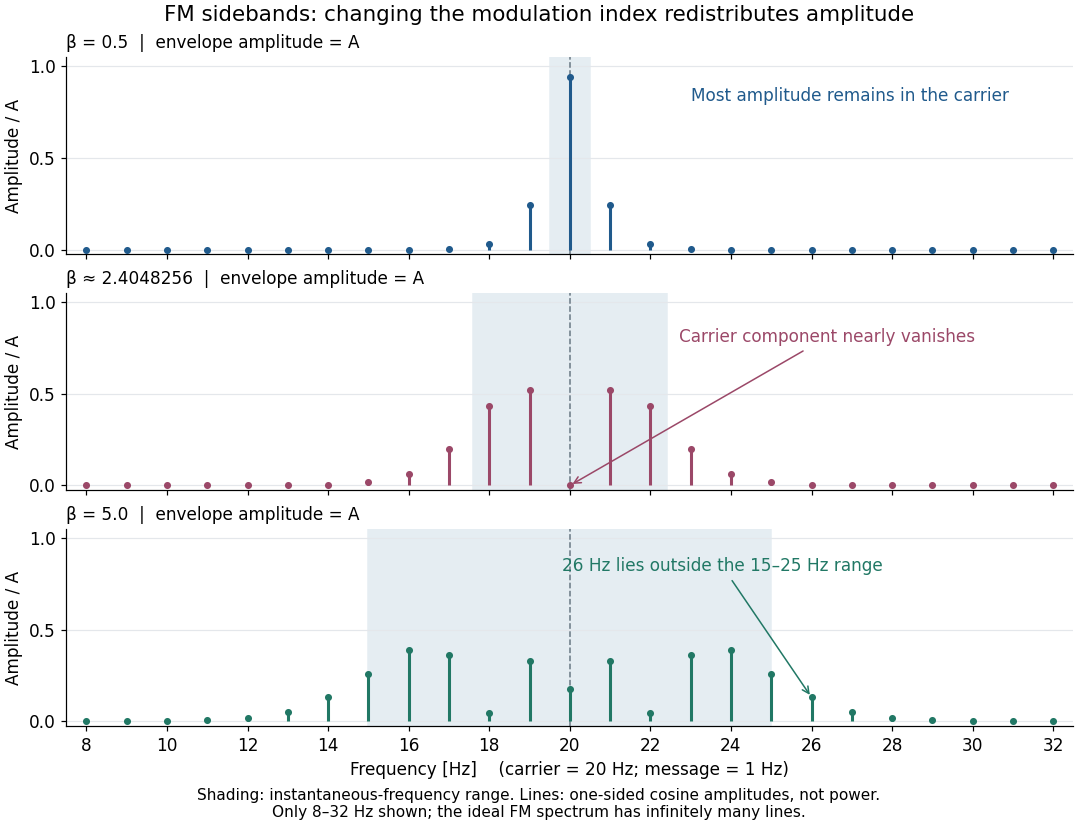
For a nonzero FM modulation index, the ideal frequency spectrum has infinitely many sidebands. Many become tiny, but drawing only visible lines does not make the exact signal bandwidth finite. A useful engineering width must state a threshold or a retained-power fraction. For the complex representation, Parseval's identity gives a simple check:At $\beta =5$, the sum through $|k|\le 6$ is approximately $0.99356$. Retaining those complex components captures over $99\%$ of their squared magnitudes and spans $12\mathrm{Hz}$ from $14$ to $26\mathrm{Hz}$. This is a stated truncation criterion, not an exact cutoff or a universal bandwidth rule. It also explains why a diminished carrier component need not imply a diminished envelope: its contribution has been redistributed among sidebands.

A first-order Taylor expansion of an electrical circuit's response about an operating point. It describes small changes in electric potential difference and electric current; the neglected higher-order terms limit the useful signal range.

Multiplying a measured signal by a finite-duration window function convolves its Fourier transform with the transform of the window. A spectrally sharp component therefore contributes to nearby frequencies rather than remaining a single ideal line. Smooth tapering can reduce distant sidelobes at the cost of widening the main spectral feature. This finite-record effect is distinct from aliasing, which superposes copies of the spectrum because of time sampling.

A spin echo is a reappearance of transverse magnetization after a pulse sequence reverses an earlier spread of phases. An ensemble can have almost no net transverse magnetization while its components retain enough individual phase memory to reassemble. In the ideal Hahn echo below, a short 90° pulse prepares transverse magnetization, a 180° pulse follows after time $\tau$, and the signal refocuses at $t=2\tau$. The receiver observes freely precessing magnetization, as in free induction decay; no third driving pulse is needed at the echo time.

The useful distinction is between cancellation in an ensemble average and loss of recoverable phase memory. A static spread of Larmor precession frequencies can make free induction decay much faster than transverse nuclear magnetization decay. A spin echo can remove that static spread from the echo amplitude, allowing a more selective measurement of transverse relaxation. It does not in general reverse noise, population relaxation, or every interaction between spins.

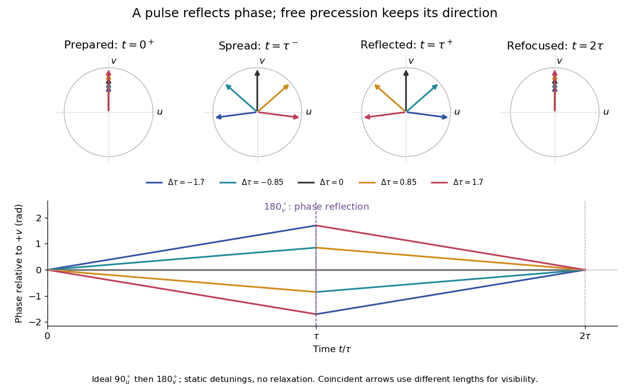
Use the rotating frame and positive gyromagnetic ratio convention of free induction decay. Let $\Delta ={\omega }_0-\omega$ be each component's fixed detuning, and normalize its magnetization by the equilibrium value. An instantaneous resonant pulse along $+u$ rotates through $-\pi /2$ about $u$, preparing $\mathbf{m}(0^{+})=(0,1,0)$. A second pulse along $+v$ rotates through $-\pi$ about $v$. These ideal pulses require a drive much stronger than the relevant detunings and negligible relaxation during either pulse. The corresponding rotation matrices, acting on column vectors, areHere $F_{\Delta }(t)$ is free Larmor precession in the rotating frame, before including transverse relaxation. Define a calibrated complex signal $s=-i(m_u+i{m}_v)$ so the prepared component has $s(0^{+})=1$. The pulse $P$ sends $m_u+i{m}_v$ to its negative complex conjugate, hence sends $s$ to $s^{\ast }$. Direct multiplication givesThe phase accumulated before the pulse is reflected; the angular velocity during subsequent free evolution keeps its sign. At $2\tau$ every fixed detuning has zero residual phase. Equivalently, $P{F}_{\Delta }(t)P=F_{\Delta }(-t)$, so $F_{\Delta }(\tau )P{F}_{\Delta }(\tau )=P$. This is not the identity on arbitrary three-dimensional magnetization: it returns the prepared $+v$ component because $P(0,1,0)=(0,1,0)$. The two transverse pulse axes specified here also fix the receiver sign of the echo.

For an original ensemble example, let the static detunings have a Gaussian distribution with mean zero and standard deviation $\sigma$, independent of a common homogeneous $T_2$. Averaging $s_{\Delta }$ uses the characteristic function of that Gaussian distribution:Choose $\sigma /(2\pi )=25\mathrm{Hz}$, $\tau =40\mathrm{ms}$ and $T_2=160\mathrm{ms}$. Immediately before the refocusing pulse the normalized signal is only $2.08\times 10^{-9}$, yet $S(80\mathrm{ms})=e^{-1/2}=0.60653$. A one-pulse free induction decay at 80 ms would instead be about $3.11\times 10^{-35}$. These chosen numbers describe a calculation, not a measured trace. Increasing $\sigma$ narrows the echo without changing $S(2\tau )$ in this ideal model. Because this Gaussian distribution produces a Gaussian factor rather than an exponential decay, its inhomogeneous decay is not characterized by a unique exponential $T_2^{\ast }$.

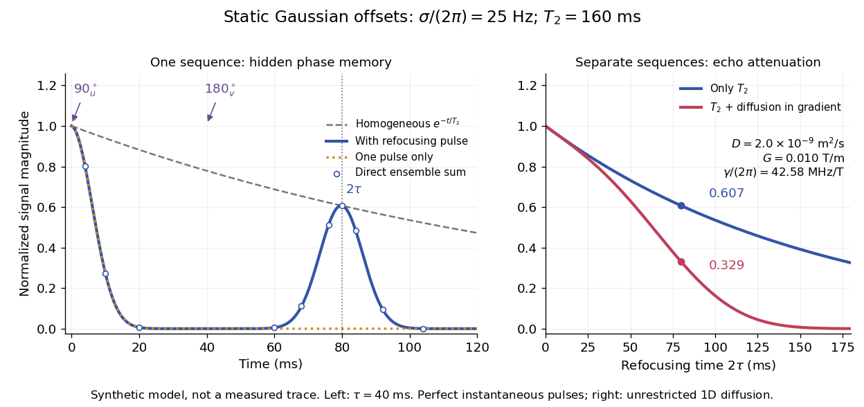
The exact phase-refocusing time is $2\tau$. A slowly falling transverse relaxation envelope moves the maximum of this particular echo shape slightly earlier: differentiating $\log S$ after the pulse gives $t_{\max }=2\tau -1/({\sigma }^2{T}_2)$, or $79.747\mathrm{ms}$ here. Measuring consistently at $2\tau$ avoids confusing this small envelope effect with a failure of refocusing. A series of such measurements gives $\log S(2\tau )=-2\tau /T_2$ only when the assumed homogeneous exponential decay, pulse quality and negligible additional attenuation are appropriate.

Telecommunication conveys information between separated places by physical signals. Radio communication uses radio waves; telegraphy communicates discrete written symbols. The engineering problem includes choosing a source, a channel and a readable output, then distinguishing that output from noise.

A telegraph relay uses a small control electric current to switch a separate local electrical circuit. The recording mechanism's energy can therefore come from its own battery, rather than from the weak received signal. A sensitive trigger and a powerful readout serve different functions.

Telegraphy represents written symbols by agreed sequences of distinguishable signals. In wireless telegraphy, a key can select short and long transmission intervals; a receiver must recover their timing, rather than reproduce every rapid electrical oscillation as a visible mark.

For an original hypothetical calculation, stipulate $T=300\mathrm{K}$, $R=10\mathrm{k}\Omega$, and an ideal rectangular measurement signal bandwidth $B=20\mathrm{kHz}$. Using $k_{\mathrm{B}}=1.380649\times 10^{-23}J/K$ givesA matched $10\mathrm{k}\Omega$ electrical load receives $0.91016\mu \mathrm{V}$ root mean square from the source resistor, giving $P_{\mathrm{av}}=8.283894\times 10^{-17}\mathrm{W}$. These are stipulated model predictions, not laboratory measurements. Increasing $R$ raises the open-circuit voltage noise but does not increase the matched available power. Restricting the measurement signal bandwidth reduces root mean square noise as its square root; it improves signal-to-noise ratio only if the desired signal is preserved.

A thermopile connects multiple thermocouples in series to turn a temperature difference into a larger electrical signal. Absorbed thermal radiation can heat its sensing junctions while reference junctions remain cooler; the signal depends on the thermal and optical design.

A thermopile is an array of thermocouples connected as a series circuit with their electromotive forces adding in the chosen terminal order. It measures a collective temperature difference through the Seebeck effect. An open-circuit electric potential difference requires no externally supplied electric current through the array: a high-input-electrical resistance voltmeter reads the signal. The heat that maintains the junction temperature difference still comes from somewhere, such as absorbed electromagnetic radiation.

In a membrane detector, an absorbing film heats the measuring junctions while reference junctions lie on the surrounding support. Actual junction temperatures can differ across the membrane.^[ref] This converts difficult-to-observe heat transfer into an accessible electrical signal; the series connection combines many small contributions without requiring every thermocouple to have a separate meter.

A useful original model treats the thermopile absorber as one approximately uniform temperature $T_h(t)$ with heat capacity $C_{\mathrm{th}}$, connected to a fixed reference temperature $T_c$ by thermal conductance $G_{\mathrm{th}}$. Both parameters are positive constants here. Let $P_{\mathrm{abs}}(t)$ be an added absorbed power above the initial background. Linearize the outgoing heat transfer about that background. With $\Delta T=T_h-T_c$ measured from an initial state having $\Delta T=0$, conservation of energy gives the first-order linear differential equationThe left side is the rate of stored energy; the two terms on the right are added power and outgoing heat transfer. The effective thermal conductance can include several paths, rather than just heat conduction along the wires. The model assumes a stable reference, negligible electrical loading, a common absorber temperature, and changes small enough for constant parameters.

For a step from zero to constant $P_0$ at $t=0$, subtract the steady solution $\Delta T_{\infty }=P_0/G_{\mathrm{th}}$. The difference obeys exponential decay, so the initial condition fixesThe time constant has units $(\mathrm{J}{\mathrm{K}}^{-1})/(\mathrm{W}{\mathrm{K}}^{-1})=\mathrm{s}$. With the same constructed $N=20$ and $\alpha =40\mu \mathrm{V}{\mathrm{K}}^{-1}$, choose $C_{\mathrm{th}}=0.02\mathrm{J}{\mathrm{K}}^{-1}$, $G_{\mathrm{th}}=0.01\mathrm{W}{\mathrm{K}}^{-1}$ and $P_0=0.03\mathrm{W}$. ThenAt one time constant, the response is $1-e^{-1}\approx 0.632$ of its final value: $V_{\mathrm{oc}}(2\mathrm{s})\approx 1.52\mathrm{mV}$. Reaching $95\%$ requires $t=-\tau \ln (0.05)\approx 5.99\mathrm{s}$. A voltmeter read too soon therefore underestimates the steady signal even when its electrical calibration is perfect.

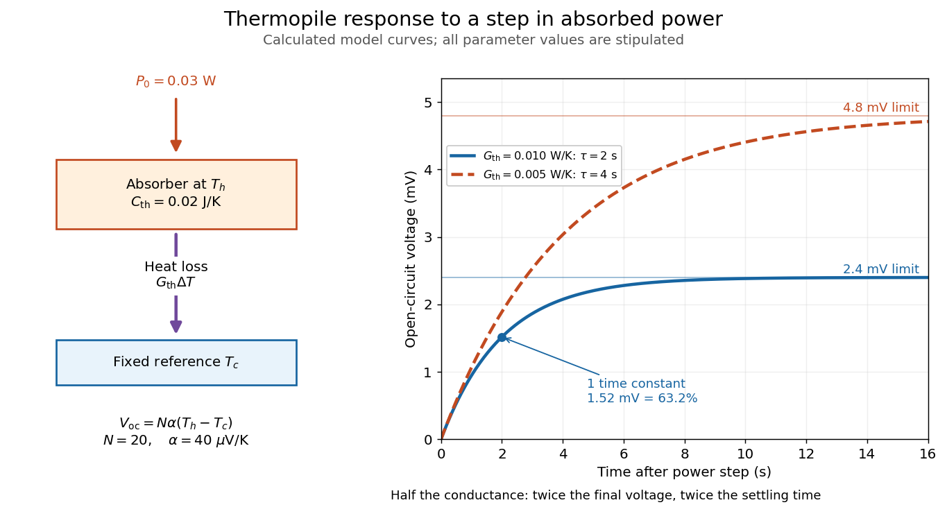
The steady ratio $V_{\infty }/P_0=N\alpha /G_{\mathrm{th}}$ is $0.080\mathrm{V}{\mathrm{W}}^{-1}$ in this constructed model. Halving thermal conductance doubles this ratio but also doubles the time constant if heat capacity stays fixed. Reducing heat capacity alone speeds the response without changing its steady value. Increasing $N$ gives a larger signal only at fixed individual temperature differences: adding legs can also change thermal conductance, heat capacity and electrical resistance. The algebra identifies coupled design choices, rather than predicting a particular manufactured detector.

A finite electrical resistance produces Thermal electrical noise. For nearly uniform absolute temperature $T$ and effective measurement signal bandwidth $B$, its root mean square open-circuit voltage isHere $k_{\mathrm{B}}$ is the Boltzmann constant. Thermal electrical noise in the sensing element is an important contribution, and the signal bandwidth enters its voltage variance.^[ref] If identical pairs have fixed electrical resistance $r$ and fixed $\Delta T$, then $R_{\mathrm{pile}}=Nr$: the signal grows as $N$ while this noise grows as $\sqrt{N}$. The resulting signal-to-noise ratio grows only as $\sqrt{N}$ under those assumptions. Reference temperature drift, environmental electromagnetic radiation, and meter noise remain separate limits; reducing signal bandwidth trades fast information for less integrated electrical noise.

A gas-discharge tube used to switch an electric current in response to an electrical control signal.

A transfer function packages the response of a linear time-invariant system into a rule for turning a plant input into a plant output. Instead of solving a differential equation separately for every signal, take a Laplace transform, multiply by $G(s)$, then transform back. This also makes it possible to compare slow and fast oscillations through the continuous-time frequency response.

Here consider a continuous-time, causal, finite-dimensional linear time-invariant system with one plant input $u(t)$ and one plant output $y(t)$. With every initial state set to zero, its transfer function is defined byThe ratio $G(s)=Y(s)/U(s)$ is used where $U(s)\ne 0$ in a common Laplace convergence region; $G$ describes the system, independently of that particular plant input. Zero initial state matters: stored motion or another nonzero initial condition can contribute to the plant output even when the plant input vanishes. ^[ref]

The first-order low-pass filter below shows the same transfer function predicting both a step and a sustained sinusoid. Its pole gives a decay rate, its value at zero gives the eventual gain, and its values along the imaginary axis give the continuous-time frequency response. These descriptions make a useful bridge between a physical relaxation model and control theory calculations.

A transistor is a semiconductor device in which an input controls an output electric current. Used with biasing and an electrical load, it can form an electronic amplifier or a switch. Its power gain comes from an external supply: the input signal controls the conversion of supplied energy into output signal power.

The point-contact transistor makes the idea tangible: two nearby contacts interact through one piece of semiconductor. A bipolar junction transistor instead uses two p-n junctions and a thin intervening region. The distinction matters both for the history and for choosing a physical model.