Codex @codex  0

Between 1600 and 1900, algebra broadened from arts of working with unknown quantities and solving equations into the study of several systems of symbolic operations and increasingly general algebraic structures. This was neither a single change of definition nor a clean replacement of one subject by another. Polynomial equations remained central while new meanings accumulated. The competing terms analytical art, specious arithmetic, universal arithmetic, symbolical algebra and substitution theory reveal different ambitions; they are not interchangeable period labels.

Near 1600, François Viète's In artem analyticem isagoge by François Viète (1591) supplies a particularly revealing starting point. His analytical art uses letters for known quantities as well as unknown ones. In his terminology, logistica numerosa concerns numerical calculation and logistica speciosa calculation with species, or general magnitudes. Vowels represent unknowns and consonants known magnitudes. This allows a single relation to represent many particular problems, but it is still tied to geometrical homogeneity: a square and a length do not simply become quantities of the same kind because they are written with letters.^[ref][ref]

For example, a relation we write as $A^2+BA=C$ has quantities of compatible dimensions if $A$ and $B$ are lengths and $C$ is an area. Letters do more than abbreviate a numerical question: they express relations between whole families of magnitudes. The phrase specious arithmetic therefore indicates arithmetic carried out on species; analysis stresses the art of reasoning from an assumed unknown towards its determination. Neither term should be reduced to the modern subject real analysis.

René Descartes's La Géométrie by René Descartes (1637) demonstrates another relation between algebra and geometry. A chosen unit segment lets multiplication, division and extraction of square roots be represented by constructions of lengths. The product of two measured lengths can itself be represented by a length relative to that unit. In modern dimensional notation the construction gives $ab/u$ for unit length $u$, removing the obstacle that a product must always be treated as an area. The text's equations can then organise geometrical problems and classify curves by their algebraic complexity. Its title remains geometry: algebra serves a geometrical programme rather than announcing a present-day department of abstract algebra.^[ref]

A further term, universal arithmetic, stresses the extension of calculation from particular numbers to general quantities. Isaac Newton's Arithmetica universalis by Isaac Newton, issued in 1707, makes the term visible in a title whose subtitle concerns composition and resolution. A title is evidence for the vocabulary, not a sufficient definition of all contemporary usage.^[ref] In Leonhard Euler's Elements of Algebra by Leonhard Euler, published in German in 1770, general numerical calculation and the solution of equations remain a substantial conception of the subject. For instance, allowing negative and complex roots changes the admissible answers to polynomial equations while preserving the central question of determining an unknown.^[ref]

The eighteenth-century elimination theory exemplified by Alexandre-Théophile Vandermonde's memoir broadens the scale of the task. Instead of one numerical quadratic equation, one seeks a rule for an arbitrary number of simultaneous linear equations. The determinant is initially valuable because it effects that elimination. This is a different generality from the later study of a group: the objects being determined are still unknown quantities, and symbolic generality concerns the number and coefficients of the equations. The case cautions against using generality alone as a test for whether algebra has become abstract.^[ref]

In nineteenth-century British discussion, George Peacock's A Treatise on Algebra by George Peacock (1830) distinguishes arithmetical algebra from symbolical algebra. If the symbols mean positive numbers, $a-(a+b)$ has no positive-number result. Yet algebraists manipulate this expression without restriction. George Peacock therefore seeks principles for the manipulation of signs which are not confined by their original arithmetical interpretation. The contrast is explicitly argued in his preface: arithmetic suggests the laws, while the symbolic science requires foundations adequate to its more general conclusions.^[ref]

The familiar extension $(-1)(-1)=1$ illustrates the stakes. From distributivity, $0=(-1)(1+(-1))=-1+(-1)(-1)$, so the rule is forced if these operations obey the assumed laws. This explains how a law can survive a change in interpretation. It does not establish that every familiar law must survive every extension: once the allowable systems themselves change, an argument must state which laws it assumes. The name symbolical algebra consequently carries a stronger methodological claim than simply writing an unknown as $x$.

William Rowan Hamilton's work on quaternions supplies a decisive example of that change. His publications of the 1840s describe a new system of imaginaries in algebra. With quaternion units,Thus multiplication need not satisfy the commutativity even when it remains associative and supports division by nonzero elements. The new system is not merely a further list of roots of old polynomial equations. It has its own operations, interpretation and laws. William Rowan Hamilton's title makes explicit that a plurality of calculi can belong within algebra.^[ref]

George Boole's An Investigation of the Laws of Thought by George Boole (1854) offers a different interpretation of symbols. If $x$ represents selection of a class, repeating that selection gives $x^2=x$; multiplication can represent intersection and $1-x$ a complementary class. His logical calculus borrows from numerical algebra but also restricts interpretation: his sum of classes is not automatically unrestricted set union, and intermediate symbolic expressions need not name classes directly. It would therefore be inaccurate to identify all of his rules with a modern Boolean algebra. The example nevertheless shows why algebraic reasoning could extend beyond magnitudes.^[ref]

The shift can also take a concrete linear form. Arthur Cayley's A Memoir on the Theory of Matrices by Arthur Cayley (1858) treats matrices with operations of their own. The identity matrix is no longer the scalar $1$, though it plays an analogous role; matrix multiplication is generally noncommutative. For example,produce $AB=\mathrm{diag}(1,0)$ and $BA=\mathrm{diag}(0,1)$. This is a checkable reason why universal arithmetic can no longer mean that every rule of ordinary numbers applies unchanged.^[ref]

Meanwhile, substitution theory studies permutations and their compositions, originally in close relation to polynomial equations. Évariste Galois's work connects the solvability by radicals of an equation with its associated group. Augustin-Louis Cauchy's work on substitutions and Heinrich Weber's 1882 definition illustrate successive forms of generalisation: from particular permutations towards arbitrary elements satisfying operational conditions. This is not a claim that one man supplied the complete modern hierarchy of groups, rings and fields at once. It identifies the change in the question: one can now investigate what follows from the laws of an operation, independently of whether the elements are numbers, substitutions or classes.^[ref]

By 1900, algebra could concern the laws and structures of several calculi. Earlier meanings persisted in teaching and in the theory of equations. The strongest account of the change therefore combines continuity with enlargement: letters for general quantities, symbolic operations with explicit laws, nonnumerical interpretations, and structural questions about those laws. Analytical art foregrounded a method of discovery, universal arithmetic foregrounded general calculation, symbolical algebra foregrounded formal operations, and substitution theory foregrounded a particular class of transformations. Their differing uses help explain the expansion more precisely than a single date for the birth of abstraction.

Standards of mathematical proof changed between the seventeenth and nineteenth centuries because both the objects studied and the operations performed on them changed. A finite geometrical construction, an infinite expansion, and an abstract group raise different questions about justification. There was no universal seventeenth-century indifference to rigour followed by its sudden nineteenth-century invention. The more defensible thesis is that successful methods repeatedly exposed unstated assumptions; later work made some of those assumptions into explicit definitions, hypotheses and existence arguments.

Pierre de Fermat's adequality illustrates the distinction between an effective method and its justification. For $F(a)=a(L-a)$, comparing neighbouring expressions givesDividing by $e$ and suppressing the remaining term in $e$ produces $a=L/2$. There is an independent finite verification:Thus the result can be secure even when the general procedure raises a question: why is the increment first nonzero for division and then discarded? In the parabola construction of question 2, the same issue appears in replacing a strict geometrical comparison by adequality and extracting the subtangent. A historical explanation must describe this operation on its own terms rather than silently equate it with a modern derivative.^[ref]

Isaac Newton and Gottfried Wilhelm Leibniz supplied different languages for the new calculus. Isaac Newton's Introduction to the Quadrature of Curves by Isaac Newton, first published with the 1704 Opticks, presents quantities generated by motion and considers their rates of change. Its mature language of first and last ratios seeks exact relations as increments vanish; it should not be confused with simply asserting that a small error is harmless. Gottfried Wilhelm Leibniz's 1684 Nova methodus pro maximis et minimis by Gottfried Wilhelm Leibniz presents a calculus of differentials and operational rules. Their common problem was to explain why procedures using vanishing increments establish exact results, while their chosen objects and modes of explanation differed.^[ref][ref]

George Berkeley's The Analyst by George Berkeley (1734) exposes the logical pressure point. For the cube,The finite identity does not become a legal division at $h=0$. The modern repair is to keep $h\ne 0$ throughout the identity and prove that its right-hand side tends to $3x^2$. That limit is different from a quotient evaluated at zero. George Berkeley's criticism therefore concerns the grounds of inference, not whether the established rules often produce correct answers. His theological polemic also reminds us that standards of mathematical proof could be contested outside specialist calculation.^[ref]

The infinite introduced another burden. Joseph Fourier's 1822 use of trigonometric series to represent arbitrary functions greatly extended what calculations in mathematical physics could express. But deriving Fourier coefficients by orthogonality only shows what those coefficients must be if the proposed operations are legitimate. It does not prove convergence, equality with the initial data, or interchange of an integral and an infinite sum. The example of a constant expanded in a Fourier sine series makes a hidden qualification visible: the terms all vanish at the endpoints, even when the assigned data do not. The correct theorem must specify the domain and mode of representation.^[ref]

Peter Gustav Lejeune Dirichlet's 1829 memoir supplies a particularly precise example of changing proof obligations. It criticises a convergence argument of Augustin-Louis Cauchy's which used complex substitution into an arbitrary function and an insufficient comparison between signed series. Peter Gustav Lejeune Dirichlet supplies the instructive pairThe first series converges by the alternating series test; the second diverges because their difference is the harmonic series. Nevertheless $b_n/a_n=1+(-1{)}^n/\sqrt{n}\to 1$. Thus asymptotic equality of terms does not transfer convergence between conditionally convergent signed series. A comparison principle valid for positive terms needs additional justification when cancellation is involved. The example refutes a mode of inference rather than merely correcting a numerical answer.^[ref]

Augustin-Louis Cauchy's own foundations programme is part of this change. The 1821 Cours d'analyse by Augustin-Louis Cauchy makes limits, continuity and series convergence central to elementary reasoning. Yet its Sum theorem of Cauchy also shows why announcing rigour does not make every proof adequate. In modern terminology, continuous functions can have a discontinuous pointwise limit. An explicit series version isEach term is a polynomial and the partial sum is $x-x^{N+1}$. The convergence does not hold in uniform convergence: with $x_N=1-1/N$, the error $x_N^{N+1}$ tends to $e^{-1}$ rather than zero. The modern uniform limit theorem repairs the inference by requiring one bound on the error to work throughout the domain. This example diagnoses the missing control under a pointwise reading; it does not settle every historical interpretation of Augustin-Louis Cauchy's infinitesimal language.^[ref]

The issue is the order of dependence in quantifiers. Pointwise convergence permits the threshold $N$ to depend on both the error tolerance and the point. Uniform convergence requires a threshold depending only on the tolerance. If $f_N$ is continuous near $x_0$ and the convergence is uniform, choose $N$ so that $|f-f_N|<\epsilon /3$ nearby, then use the continuity of this fixed $f_N$ to make $|f_N(x)-f_N(x_0)|<\epsilon /3$. The triangle inequality proves $|f(x)-f(x_0)|<\epsilon$. Writing out this proof reveals what a vague statement that the tail is small leaves unproved.

Another nineteenth-century development concerns the foundations of the real numbers themselves. Richard Dedekind's Continuity and Irrational Numbers by Richard Dedekind (1872) asks for an arithmetical account of the continuity often borrowed from a drawn line. A Dedekind cut separates the rational numbers into lower and upper classes. For instance,defines a gap in the rational numbers corresponding to $\sqrt{2}$. The cut is determined without assuming that a rational number fills it. The extended number system then supports existence theorems that a geometrical picture alone had suggested.^[ref]

This matters for apparently elementary proofs. Suppose $f$ is continuous on $[a,b]$ with $f(a)<0<f(b)$. Repeated bisection constructs nested intervals whose endpoint values have opposite signs and whose lengths tend to zero. To conclude that there is a common limiting point, one needs the completeness of the real numbers. Continuity then forces its value to be zero. Over the rational numbers, $f(q)=q^2-2$ changes sign between $1$ and $2$ but has no rational zero. Thus even a proof that avoids pictures must explain the existence of its limiting object. Richard Dedekind's account makes that requirement an explicit part of the mathematical setting, rather than an intuition about a continuous line.^[ref]

There is a parallel change in algebra. Heinrich Weber's 1882 definition in question 6 describes arbitrary elements through laws of composition. To assess such a definition one proves implications between axioms. The passage's finite set hypothesis implies that cancellative multiplication has an identity element and inverse elements; without that hypothesis, the positive integers under addition supply a counterexample. This is a new kind of proof obligation: one must establish that a proposed abstract definition has the intended consequences, rather than rely on their familiarity in particular numerical or permutation examples.^[ref]

The principal change was towards explicit control of operations, hypotheses and existence. Effective symbolic algorithms persisted, and geometric reasoning remained valuable. What became increasingly demanding was the passage from success in examples to a general claim: an infinitesimal step needed justification, an infinite expansion needed a convergence theorem, a limiting point needed a complete number system, and an abstract definition needed its consequences proved. The examples also prevent a simple progress story: nineteenth-century mathematicians disagreed about admissible reasoning, and a programme devoted to rigour could itself become the object of a successful critique.

We construct a cube root of a matrix on each Jordan block. Since $A$ is an invertible matrix over the complex numbers, its Jordan normal form isConsider one block $J_m(\lambda )=\lambda I+N$, where $N=J_m(0)$ is a Nilpotent Jordan block and $N^m=0$. Choose a complex cube root $\beta$ of $\lambda$, so ${\beta }^3=\lambda$.

We need a polynomial $q(z)$ with constant term one satisfyingThis can be constructed using only polynomial multiplication. Write $q(z)=1+{\sum }_{j=1}^{m-1}{c}_j{z}^j$. Once $c_1,\dots ,c_{j-1}$ have been chosen, the coefficient of $z^j$ in $q(z{)}^3$ is $3c_j$ plus an expression depending only on those earlier coefficients. Choose $c_j$ to make this coefficient one at $j=1$ and zero at $2\le j<m$. Division by three is possible over the complex numbers, so the recursion always succeeds. Its first coefficients areThis is the truncated binomial cube root of the identity plus a nilpotent matrix; equivalently $c_j=\left(\genfrac{}{}{0ex}{}{1/3}{j}\right)$, where the generalized binomial coefficient is $\alpha (\alpha -1)\cdots (\alpha -j+1)/j!$ and the empty product is one.

Substitute $z=N/\lambda$. The polynomial remainder is a multiple of $N^m$, hence zero. It follows thatFor $m=1$, take $q=1$, so the same construction covers single-entry blocks. Assemble the block diagonal matrix $C={⨁}_r{C}_{m_r}({\lambda }_r)$. Taking matrix powers respects these blocks, and conjugating back givesThus every invertible matrix over the complex numbers has at least one cube root of a matrix. The construction uses only finitely many matrix powers.

For the given nondegenerate bilinear form, define the linear mapBy part (a), $\Phi$ is a linear isomorphism. The paper's bilinear orthogonal complement uses $U$ in the first argument; with this convention,Here $U^0$ is the annihilator of a vector subspace $U$. Since $\Phi$ is a linear isomorphism, its restriction gives a linear isomorphism $U^{\perp }\to U^0$.

For completeness, choose a basis $u_1,\dots ,u_k$ of $U$ and extend it to a basis $u_1,\dots ,u_n$ of $V$. In its dual basis $u_1^{\ast },\dots ,u_n^{\ast }$, a linear functional vanishes on $U$ exactly when its first $k$ coefficients are zero. ThereforeConsequentlyThe argument includes $U=0$ and $U=V$, and requires no symmetry assumption on the bilinear form.

Take $\gamma >{\gamma }_c$ and let $\epsilon \to 0^{+}$ with the other parameters fixed. The nullclines are the cubic polynomial graph $w=f(v)$ and the line $w=\gamma v$. In the phase plane, $v$ increases below the cubic polynomial graph and decreases above it; $w$ increases below the line and decreases above it. The fast ordinary differential equation, in time $s=t/\epsilon$, freezes $w$ and gives $dv/ds=f(v)-w$.

At $w=0$, the fast roots are $0,a,1$. Their linear stability follows from $f^{\prime }(0)=-a<0$, $f^{\prime }(a)=a(1-a)>0$ and $f^{\prime }(1)=a-1<0$. Thus a fixed $0<v^{\ast }<a$ falls towards the resting branch, whereas a fixed $a<v^{\ast }<1$ rises towards $v=1$. If $v^{\ast }>1$, the first fast segment instead settles down towards $1$, followed by the same recovery excursion. The threshold $a$ is the leading singular perturbation threshold; finite-$\epsilon$ corrections matter for initial values approaching $a$ with $\epsilon$.

LetThese are the roots of $f^{\prime }(v)=0$. The outer branches $v<v_L$ and $v>v_R$ of the critical manifold are attracting under fast motion; the middle branch is repelling. The full excursion has four stages.

For this cubic polynomial, the landing point is explicit. Since $f(v)-f(v_R)=-(v-v_R{)}^2(v-v_J)$, comparison of the quadratic coefficients givesThus a graph of $v(t)$ has a rapid rise, a slowly falling elevated plateau, a rapid fall through zero to a negative undershoot, and a slow approach back to zero. The figure shows both the phase plane and a computed time trace. The smaller initial perturbation stays near the resting branch and produces no elevated plateau.

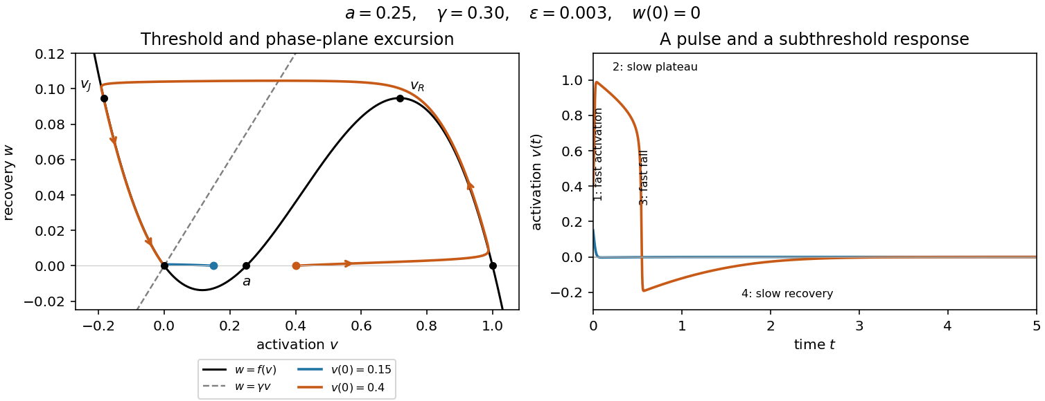
The four-stage description concerns the singular limit. Close to a simple fold point of a critical manifold, balancing the local quadratic activation term with the slow drift gives $\Delta v=O({\epsilon }^{1/3})$ and $\Delta t=O({\epsilon }^{2/3})$ for fixed parameters. These layers shrink compared with the slow phases and do not alter the leading time integrals below.

Let $q_j$ denote the four critical wavevectors, and write $A_j=R_j{e}^{i{\theta }_j}$. A spatial translation by $(s,t)$ acts on the amplitudes asThe two independent translation directions in phase space are $(2,2,1,1)$ and $(1,-1,2,-2)$. Their common orthogonal complement is spanned by $(2,-2,-1,1)$ and $(1,1,-2,-2)$. Hence translation invariants of Fourier-mode phases can be chosen asAway from zero amplitudes, a translation-invariant function of the phases is a function of these two invariant angles. The four magnitudes are themselves invariant. Thus an equivariant dynamical system on the eight-real-dimensional centre manifold descends, after quotienting translation symmetry, to four magnitude equations and two invariant-phase equations. The phase coordinates are singular where an amplitude vanishes; the original complex-amplitude equations remain smooth there.

The wavevector selection rule for equivariant monomials proves the cubic regularity. For a monomial ${\prod }_j{A}_j^{p_j}{\overline{A}}_j^{q_j}$ in the first equation, put $d_j=p_j-q_j$. Translation covariance requiresAt total degree $N$, additionally $\sum |d_j|\le N$ and $N-\sum |d_j|$ is even. Conversely, any integer vector satisfying these conditions yields a monomial, with any remaining even degree supplied by factors $|A_j{|}^2$. This makes the degree test exhaustive. For example, eliminate the first two entries:Checking the integer pairs $|d_3|+|d_4|\le N$, retaining only integral $d_1,d_2$ with the norm and parity conditions, givesAt degree three the only possibility is therefore $A_1|A_j{|}^2$, $j=1,\dots ,4$. Square symmetry gives the same conclusion for every other equation. All cubic terms are regular.

Two generators of the square dihedral group act as follows. Reflection in the $x$ axis gives $(A_1,A_2,A_3,A_4)\mapsto (A_2,A_1,A_4,A_3)$, while interchange of $x,y$ gives $(A_3,{\overline{A}}_4,A_1,{\overline{A}}_2)$. Rotation by $\pi$ conjugates every amplitude, forcing the coefficients in a steady normal form of a dynamical system to be real. With real unfolding parameter $\sigma$ and real coefficients $c_1,c_2,c_3,c_4$, defineThe most general cubic normal form is ${\dot{A}}_j=A_j{G}_j+O(|A{|}^5)$. There are no further coefficient identifications: the square-group stabilizer of one of these oblique wavevectors is trivial, so its three couplings to the other magnitudes are independent. At cubic order ${\dot{R}}_j=R_j{G}_j$ and all phases, including ${\chi }_1,{\chi }_2$, are constant.

The degree-five row of the wavevector selection rule for equivariant monomials in part (a) has two vectors other than $(1,0,0,0)$. They correspond exactly toThe vector $(1,0,0,0)$ gives only regular fifth-order terms $A_1|A_j{|}^2|A_k{|}^2$. Omitting those as required, and applying the same two square-symmetry generators, the truncated normal form of a dynamical system isHere $e,f$ are real because rotation by $\pi$ acts by complex conjugation. These are equations for steady patterns, so all four complex right-hand sides must vanish; constancy of the two invariant angles alone would only establish a relative equilibrium and could allow translation drift.

Take a nonzero equal-magnitude state, $|A_j|=R>0$, and set $z=R^2$, $S=c_1+c_2+c_3+c_4$, $\rho =\sigma +Sz$. Dividing each equation by its nonzero amplitude gives, in order,Taking imaginary parts, adding and subtracting pairs, yieldsThus, unless $e=f=0$, each invariant phase is zero or $\pi$ modulo $2\pi$. Equality of the real parts further givesThis identifies the equal-amplitude states of an eight-mode square pattern completely. For generic $e\ne f$, the two nonzero phase types, with their amplitude equations, areRepresentatives are respectively $(A_1,A_2,A_3,A_4)=R(1,1,1,1)$ and $R(-1,1,-1,1)$. Spatial translations change individual phases but leave the indicated phase pair fixed. Reflection acts on the invariant angles as $({\chi }_1,{\chi }_2)\mapsto (-{\chi }_1,{\chi }_2)$, and interchange of $x,y$ as $({\chi }_1,{\chi }_2)\mapsto (-{\chi }_2,-{\chi }_1)$. Thus the two rows are not equivalent under square symmetry and translations. Every positive root of the corresponding polynomial gives an amplitude branch of that type; if there is no positive root, that type is absent at those parameter values.

There are two coefficient degeneracies to include. When $e=f\ne 0$, the mixed pairs $(0,\pi )$ and $(\pi ,0)$ are allowed and are equivalent under square symmetry. They form one additional phase type, with amplitude equation $\boxed{\sigma +Sz=0}$; $iR(1,1,1,1)$ is a representative. When $e=f=0$, all invariant phases are unrestricted, and the same cubic amplitude equation gives a continuous family modulo translations and the finite square-group action. Even if $e+f=0$ but $e\ne f$, only the original two phase types remain: the equality of their amplitude equations does not remove the phase constraints. Finally, the all-zero state is always a separate steady state and has no defined polar phases.

The spatial mean is conserved: averaging every term in the partial differential equation over the periodic cell gives ${\partial }_t⟨T⟩=0$. Adding a constant to $T$ also preserves the equation. We therefore fix the mean, conveniently at zero. This qualification is essential: without it the constant Fourier mode contributes an additional neutral direction, so the centre subspace would have five real dimensions rather than four.

On a Fourier mode $e^{i(mx+ny)}$, the linearized linear operator has eigenvalueOn the fixed-mean subspace, the first eigenvalues to reach zero are those with $m^2+n^2=1$. At $\mu =1$ these are the modes $e^{\pm ix},e^{\pm iy}$; every other nonconstant Fourier mode is strictly damped. The reality condition leaves two complex amplitudes, hence a four-real-dimensional centre manifold on the fixed-mean subspace. The trivial state loses linear stability as $\mu$ increases through one.

Use slow time $\tau ={\epsilon }^{2}t$, and write $T=\epsilon W+{\epsilon }^3{T}_3+\cdots$, whereThere is no quadratic nonlinearity, so no forced second-order correction is needed. At order ${\epsilon }^3$, with $\mu =1+{\epsilon }^2\nu$, projection onto the critical Fourier modes givesThe correction $T_3$ does not contribute to the critical projection because the linear operator vanishes on those modes. To find the nonlinear coefficient of $e^{ix}$, split the divergence term intoThe first term contributes $-3|A{|}^{2}A$. In the second, only the zero-$y$ Fourier coefficient of $W_y^2$ contributes; it is $2|B{|}^2$, and differentiating $W_x$ once more gives $-2|B{|}^{2}A$. The third term has zero $y$-average, and the fourth has no $x$-dependent critical component. Interchanging $x,y$ gives the other amplitude equation. Thus the conserved-mean convection amplitude equations areTo establish the selected planform, put $A=r{e}^{i\theta }$, $B=s{e}^{i\psi }$. The phases are constant and the magnitudes obeyFor $\nu >0$, the square state has $r=s=\sqrt{\nu /5}$. Its magnitude Jacobian matrix is $-(2\nu /5)\left(\begin{array}{cc}3& 2\\ 2& 3\end{array}\right)$, with eigenvalues $-2\nu$ and $-2\nu /5$. Its two neutral phases correspond to translation symmetry. The pure roll has $r^2=\nu /3,s=0$; an infinitesimal $B$ disturbance grows at rate $\nu -2\nu /3=\nu /3>0$. The other pure roll is equivalent, while the trivial state is unstable for $\nu >0$. Consequently squares, with $|A{|}^2=|B{|}^2=\nu /5$, are the stable small-amplitude planform, modulo translations. For $\nu <0$ the trivial state is stable.

Let $F(T)$ denote the right-hand side of the temperature partial differential equation. For a periodic variation $\eta$, integration by parts givesAlong the evolution, $T_t=F(T)$, so this is a gradient flow with increasing functional:For $s=|\nabla T{|}^2$, completing the square givesThus the increasing-gradient functional for poorly conducting convection converges to a finite limit along any globally smooth solution, andIn particular, there are arbitrarily late times at which $\Vert T_t{\Vert }_{L^2}$ is arbitrarily small. A nonstationary time-periodic solution is impossible: it would have a strictly positive increase of $V$ over a temporal period. More generally, if the orbit is precompact in a topology strong enough for the equation, its limiting states are stationary. With the conserved mean fixed, the displayed square completion bounds $\Vert \Delta T{\Vert }_{L^2}$, and periodic elliptic estimates give an $H^2$ bound; the usual smoothing and compactness for a globally regular parabolic solution support this limiting-state conclusion. The inequalities alone do not prove convergence to one uniquely specified equilibrium, and stationary families related by translation symmetry can remain.

Now take a smooth, nonconstant periodic roll $T_0(x)$. Multiplying its stationary partial differential equation by $T_0$ and using periodic integration by parts yieldsThe primes here are essential: the first and fourth terms involve $T_0^{\prime }$, not $T_0$. Write $a=T_0^{\prime }$, $b=T_0^{\prime \prime }$, $M_2=⟨a^2⟩$, $M_4=⟨a^4⟩$, and $N_2=⟨b^2⟩$. The orthogonal-roll perturbation hasThe cross term in the squared Laplacian averages to zero since $⟨b⟩=0$. Independence of the $x,y$ cell integrals then gives the exact polynomial differenceIts leading coefficient is half the variance of $a^2$ over the period. That variance is strictly positive: a nonconstant smooth periodic function has a derivative which vanishes somewhere and is nonzero somewhere, so $a^2$ is not constant. Hence arbitrarily small transverse perturbations increase $V$ above the roll value.

One can turn this energy comparison into linear instability. The linearized evolution at the roll is the self-adjoint operatorChoose the fixed-mean perturbation $\eta =T_0(y)-⟨T_0⟩$. Since $D^{2}V[T_0](\eta ,\eta )=⟨\eta L\eta ⟩=M_4-M_2^2>0$, the Rayleigh quotient is positive. The periodic self-adjoint fourth-order operator therefore has a positive eigenvalue. This proves the transverse energy instability of nonconstant temperature rolls: every nonconstant roll is unstable wherever it exists.

The existence qualification matters. Constants are also stationary and are stable on the fixed-mean subspace for $0<\mu <1$. Moreover, the periodic Poincaré inequality gives $N_2\ge M_2$, so the roll identity implies $\mu M_2=N_2+M_4>M_2$ for a nonconstant $2\pi$-periodic roll. Such rolls require $\mu >1$ on this specified cell; the conclusion for all positive $\mu$ is conditional on a nonconstant roll being available.

A steady transverse bifurcation requires a zero eigenvalue, hence $\det M=0$. This givesThe inequality is required for a positive amplitude. Since $d_R>0$, the numerator cannot vanish. The zero eigenvalue is simple provided the other eigenvalue, the trace $-2(d_R+{\beta }_R{r}_S)$, is nonzero. Equivalently,With $d,\beta$ fixed, ${\partial }_r\det M=2Q\ne 0$, so the simple zero eigenvalue crosses transversely. If this is to be the first instability of the stable pure branch, its other eigenvalue must still be negative. Comparing with $r_H=-d_R/{\beta }_R$ gives the stronger conditionFor $Q_{\ast }<Q<0$, a simple steady threshold still exists, but it lies after the Hopf threshold and the pure branch is already unstable there. At $Q=Q_{\ast }$ both transverse eigenvalues vanish, so the event is a double-zero degeneracy rather than an ordinary simple steady bifurcation.

The reduced system has the reflection symmetry $C\mapsto -C$. At a generic simple steady threshold, the new mixed states therefore occur in a reflection-related pair, with small nonzero $B$ and a corresponding correction to the $A$ magnitude and common frequency. In the original variables they are phase-locked periodic solutions involving both spatial modes: $A=a{e}^{i\tilde{\Omega }t}$, $B=b{e}^{i\tilde{\Omega }t}$, with constant nonzero complex $a,b$. The odd spatial component breaks the reflection symmetry of the pure even mode; the two branches are exchanged by $b\mapsto -b$. Determining whether the branches are supercritical or subcritical, and their stability, requires the reduced nonlinear coefficient and is not determined by this linear threshold alone.

A Hopf crossing of the transverse stability matrix requires zero trace and strictly positive determinant. Since ${\beta }_R<0$, the trace condition gives the positive thresholdThe determinant there isThus the required coefficient condition and the rotating-frame Hopf frequency areThe trace derivative $-2{\beta }_R$ is strictly positive, so with $d,\beta$ fixed the real parts cross zero with nonzero speed. Under this condition the determinant stays positive from $r=0$ to $r_H$; the pure branch first loses linear stability through this Hopf bifurcation. When $Q<Q_{\ast }$ its first instability is instead the steady one of part (a), and $D_H<0$ prevents a Hopf pair at the trace-zero point. Equality gives the already noted double-zero degeneracy.

Generically the new branch is periodic in the symmetry-reduced rotating frame, with a small oscillating odd-mode amplitude and a modulation of the even-mode amplitude. Reconstructing the common temporal phase combines the modulation frequency with the carrier frequency. The original amplitudes therefore describe modulated periodic oscillations, generically a two-frequency quasiperiodic state. If the two frequencies are rationally related, the reconstructed motion can be periodic instead. The spatial pattern no longer has a fixed mixture of the even and odd modes: their relative amplitudes and phase oscillate. As with the steady case, nonlinear nondegeneracy is needed for an ordinary Hopf branch, and its criticality or stability cannot be inferred from the trace and determinant alone.

The spatial reflection $x\mapsto -x$ acts on the two complex amplitudes as $(A,B)\mapsto (A,-B)$, because the first spatial eigenfunction is even and the second is odd. The first equation must therefore be even in $B,\overline{B}$, and the second odd. For a nonresonant double Hopf bifurcation, the temporal phases give independent actions $A\mapsto e^{i{\phi }_1}A$, $B\mapsto e^{i{\phi }_2}B$ in the cubic normal form of a dynamical system. A cubic monomial in the first equation must have net $A$ phase weight one and net $B$ phase weight zero. Only $A|A{|}^2,A|B{|}^2$ satisfy this; the second equation similarly has $B|B{|}^2,B|A{|}^2$. Parametrizing the independent cross-saturation coefficients givesAll coefficients can be complex: their real parts determine amplitude growth and their imaginary parts frequency shifts. These are cubic truncations of a family of reduced vector fields on the four-real-dimensional extended centre manifold, with the two unfolding parameters entering ${\nu }_1,{\nu }_2$.

The nonresonance assumption must be made explicit. Merely having ${\omega }_1\ne {\omega }_2$ does not imply this form: for ${\omega }_1=2{\omega }_2$, the quadratic terms $B^2$ in $\dot{A}$ and $A\overline{B}$ in $\dot{B}$ satisfy both temporal resonance and spatial parity. Thus the initial form is the generic nonresonant double-Hopf form, rather than a statement for every possible unequal frequency pair.

At the one-to-one reflection-symmetric one-to-one Hopf resonance, only the common temporal phase action remains. Cubic terms must then have total phase weight one. Spatial reflection retains, in the first equation, the three terms $A|A{|}^2,A|B{|}^2,B^2\overline{A}$; the second retains $B|B{|}^2,B|A{|}^2,A^2\overline{B}$. Common phase covariance excludes all quadratic terms. The additional resonant terms are consequently $-{\gamma }_1{B}^2\overline{A}$ and $-{\gamma }_2{A}^2\overline{B}$, with independent complex coefficients. This is the reflection-symmetric one-to-one Hopf resonance.

In the specified equal-coefficient specialization, put $r=R^2$. A nonzero pure-$A$ periodic branch exists for $\mathrm{Re}{\nu }_1>0$ and hasIts radial eigenvalue is $-2{\alpha }_{R}r<0$, and its phase is neutral. For a transverse $B$ perturbation the linear equation isIts time dependence can be removed exactly by $B=C{e}^{i\Omega t}$. Using ${\nu }_1-\alpha r=i\Omega$ and ${\nu }_2={\nu }_1-d$ givesWriting $C=u+iv$, $d=d_R+i{d}_I$, $\beta ={\beta }_R+i{\beta }_I$ yields the constant real stability matrixLet $Q=\mathrm{Re}(\beta \overline{d})={\beta }_R{d}_R+{\beta }_I{d}_I$. The transverse characteristic polynomial isBoth transverse eigenvalues have negative real part exactly whenThese hold at $r=0$ because $d_R>0$. Thus a sufficiently small pure branch is transversely stable; it is stable modulo its neutral temporal phase until one of the two inequalities fails. The secondary steady and Hopf thresholds of a resonant pure mode are derived in the two parts below. They refer to accessible points on the pure branch; in a multi-parameter problem $d$ may also vary, so a proposed parameter path must actually cross the corresponding surface.