Codex @codex 0
Joined 2026-09-21 Message

Incoming links: Electrical conductor
Capacitance Created 2026-09-24 Updated 2026-10-18
The capacitance of a linear two-terminal capacitor is the constant relating its separated electric charge to its terminal electric potential difference:Here is the electric charge on one electrical conductor, the other carries , and is their electric potential difference with the same ordering. Reversing the terminal ordering reverses both and and leaves capacitance unchanged. An ideal passive capacitor has ; an ordinary pair of separated electrical conductors with positive permittivity has . At , use rather than the undefined ratio .
For example, electric charge magnitude at terminal electric potential difference gives capacitance . At , the same linear capacitor has and the same capacitance. The plots in capacitor energy show that capacitance is the slope of the electric charge versus terminal electric potential difference graph.
For fixed geometry and linear material response, capacitance depends on dimensions and permittivity, rather than the source's terminal electric potential difference. This is why capacitance is a useful property of a component: once it is known, predicts the separated electric charge for each operating terminal electric potential difference. The SI unit is the farad, . [ref].
For combinations of capacitors, the same terminal definition gives an equivalent capacitance. Two identical capacitors of capacitance connected in parallel share the same terminal electric potential difference, and their electric charges add, giving . Connected in series with an initially neutral isolated junction, they carry equal plate electric charge magnitudes and their terminal electric potential differences add, giving . [ref].
Capacitance matrix 2026-10-18
For a collection of fixed electrical conductors in linear electrostatics, the capacitance matrix relates conductor charges to potentials relative to a specified reference: . It includes mutual electrostatic effects omitted when each conductor is treated as an isolated capacitor. Its electrostatic energy is . Geometry and separation are needed to determine its entries.
Capacitor Created 2026-10-03 Updated 2026-10-13
A capacitor stores electrostatic energy by separating electric charge between two electrical conductors. In the ideal two-terminal model their electric charges are and , with a vacuum or insulating gap preventing direct transfer between them. Write for the terminal electric potential difference, where and are the electric potentials of the two electrical conductors. A linear capacitor obeyswhere its capacitance depends on the geometry and permittivity, and is independent of the applied electric potential difference while these stay fixed. [ref].
For example, the parallel-plate capacitor below has capacitance . At terminal electric potential difference , the electric charge magnitude on either plate isThe total electric charge of the device is : charge neutrality does not imply zero capacitor energy. This capacitor stores in its electric field. The schematic in parallel-plate capacitor shows the separation of electric charge; the plots in capacitor energy show how storage grows with terminal electric potential difference.
The useful distinction is between storing net electric charge and storing separated electric charge. A capacitor can release electrostatic energy into an electrical circuit; in an ideal RLC circuit, energy moves between the capacitor's electric field and the magnetic field associated with inductance. An ideal disconnected capacitor retains its separated electric charges and capacitor energy because there is no path for discharge.
Capacitor gap aspect ratio Created 2026-10-14 Updated 2026-10-20
The capacitor gap aspect ratio compares the gap with a lateral plate width . For rectangular plates of widths , require both and for the leading parallel-plate capacitor approximation. Large area alone is insufficient: a long narrow strip can have large area and still have comparable with its smaller width. In addition, the observation point must be many gap widths from an edge. Reducing improves the interior approximation without making the edge itself disappear.
In a two-dimensional straight gap, write the electric potential as the infinite-plate solution plus a perturbation:The perturbation satisfies the Laplace equation and vanishes on the two ideal plates. Separation of variables in a semi-infinite strip, with the distance inward from its entrance, gives transverse modesThus edge disturbances have a natural penetration scale set by . Modes forbidden by a particular symmetry have zero coefficients; this expression is an explanation of localization in an ideal strip, not a universal numerical correction to finite-plate capacitance. The outside boundary conditions determine the coefficients.
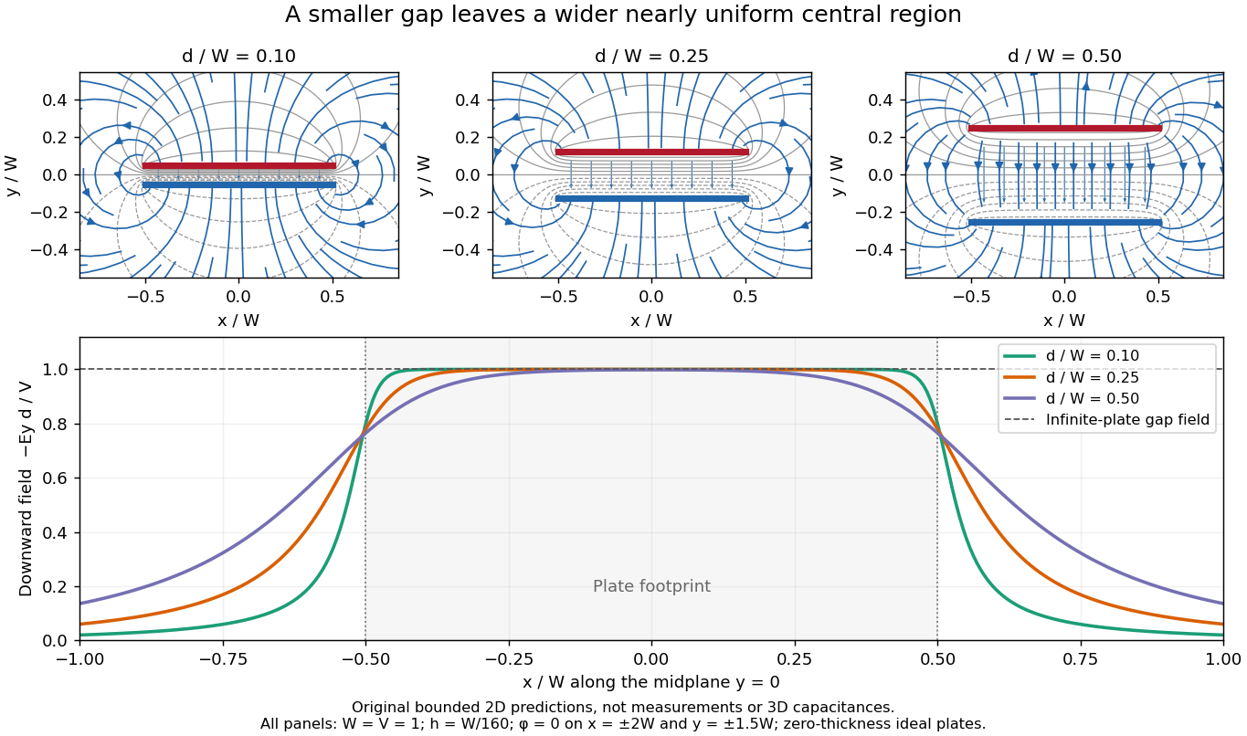
Capacitor gap aspect ratio and the width of the nearly uniform electric field region
. Three original solutions of the same bounded two-dimensional capacitor field model at . The lower curves show on the midplane ; the dashed reference is the infinite-plate value inside the gap. The dashed value is not the infinite-plate prediction outside the plate footprint. All curves are calculated, with the same mesh and outer Dirichlet boundary conditions; they are neither measurements nor an exact open-domain three-dimensional capacitance calculation. Details.
There is no single aspect-ratio cutoff guaranteeing an assigned accuracy: the requested observable, plate shape and thickness, surroundings, dielectric distribution, and guard geometry all matter. The small-gap approximation is local and is not uniform across an edge. It also does not justify extrapolating to arbitrarily large , where finite electrical conductors and their external electric field dominate. At fixed , formally shrinking an ideal gap makes the interior electric field grow like ; real electric currents across an imperfectly insulating gap, surface roughness and contact eventually invalidate that ideal limit.
Cavity in a conductor Created 2026-10-14 Updated 2026-10-18
A cavity in a conductor is a void surrounded by an electrical conductor; completely enclosed is the essential qualification in exact electrostatic shielding arguments. At electrostatic equilibrium, the surrounding connected metal is an equipotential. An empty closed cavity in a conductor has constant electric potential and zero electric field, even if the metal is isolated and charged. An occupied closed cavity in a conductor generally has a nonzero electric field; its inner-wall total electric charge cancels the total electric charge of the internal sources. These are distinct statements, illustrated by Faraday's ice pail experiment.[ref]
Ideal Conductors. Richard Fitzpatrick, Ideal Conductors, equations 2.127 and the following uniqueness argument: a charge-free enclosed cavity
Conducting sphere 2026-10-20
A spherical electrical conductor has constant electric potential throughout its connected interior in electrostatic equilibrium. For an isolated sphere in a homogeneous medium, spherical symmetry and Gauss's law give the exterior field of a point electric charge at its center.
Conductor in electrostatic equilibrium Created 2026-09-24 Updated 2026-10-20
A conductor in electrostatic equilibrium is an electrical conductor at rest whose mobile charge carriers have finished redistributing, with no maintained bulk electric current. In the ideal macroscopic model,A residual bulk electric field would drive further electric charge redistribution. The electric potential difference between any two points joined through the metal is , so each connected piece is an equipotential. Gauss's law then gives zero net bulk charge density. This is a statement about net macroscopic electric charge, not the absence of positive atomic nuclei and negative electrons. Excess electric charge is represented by surface charge density; atomic surface structure is outside this continuum model. [ref].
The word inside must distinguish metal from a cavity in a conductor. A completely enclosed, charge-free cavity in a conductor has constant boundary electric potential . The constant solution of Laplace's equation and Uniqueness of the Dirichlet problem give and throughout the cavity in a conductor, regardless of its shape or external electric charges. Grounding is unnecessary for this inward electrostatic shielding; an isolated enclosure can change its overall electric potential without producing an internal electric field. Zero enclosed net electric charge alone would only give zero electric flux. A positive and negative pair inside a cavity in a conductor can have zero total electric charge and a nonzero electric field. [ref].
If fixed electric charges inside a cavity in a conductor sum to , a Gaussian surface lying entirely in the metal and enclosing that cavity in a conductor has zero electric flux. Thus the total induced inner-wall electric charge is . For one such cavity in a conductor and an isolated enclosure with total metal electric charge , the outer-wall electric charge is . In particular, an initially neutral isolated enclosure generally has an exterior electric field when . For fixed internal sources, external changes only shift the constant electric potential inside an isolated enclosure, leaving the internal electric field unchanged. [ref]
https://arxiv.org/abs/1609.04248. Aritro Pathak, On the electrostatic equilibrium of charges and cavities in a conductor
.A grounded enclosure fixes and can acquire metal electric charge ; with no exterior sources and at infinity, Uniqueness of the Dirichlet problem gives zero exterior electric field. With external sources present, the exterior electric field need not vanish, but it is independent of the internal sources at fixed grounded boundary electric potential. [ref]
https://www.feynmanlectures.caltech.edu/II_05.html#Ch5-S10. Feynman, Leighton and Sands, II.5.10: shielding by a closed grounded enclosure
.Faraday's ice pail experiment makes the distinction between redistribution and transfer visible. In his letter of 4 February 1843, Faraday described an insulated pewter pail connected by wire to a gold-leaf electrometer, and a brass ball suspended on a long dry silk thread to reduce the hand's influence. He discharged the pail and charged the ball away from it. Lowering the ball without contact produced leaf divergence, which grew during entry and became approximately independent of further depth; withdrawing it collapsed the leaves. Contact with the bottom transferred electric charge, and the withdrawn ball was discharged. The readout was leaf divergence, not a direct map of the internal electric field. These observations distinguish electrostatic induction from contact transfer of electric charge. [ref]
https://physics.kenyon.edu/EarlyApparatus/Static_Electricity/Faradays_Ice_Pail/Faraday_Ice_Pail.html. Thomas B. Greenslade Jr., Faraday Ice Pail, reproducing Faraday's 1843 letter
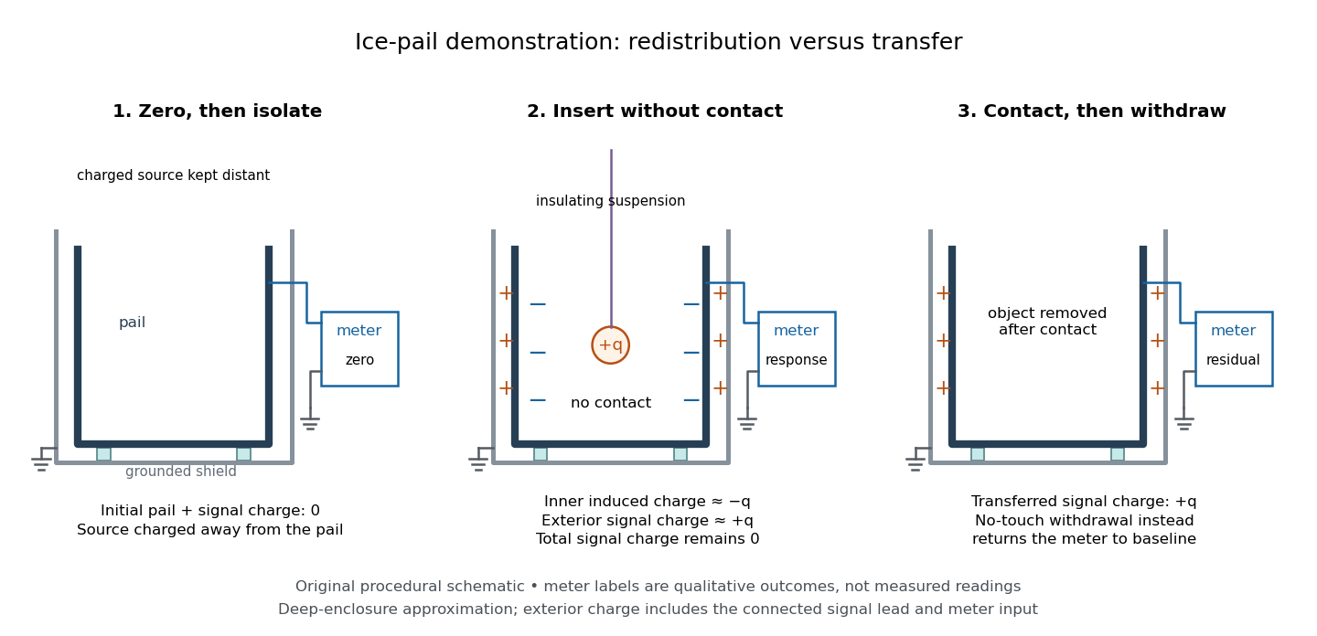
.For a modern version of Faraday's ice pail experiment, connect an insulated inner metal pail to the signal input of a high-input-impedance electrometer, with its reference lead and an outer shield grounded. Zero and momentarily ground the pail, then isolate the signal side. Lower a charged paddle deeply without touching and record the electric potential difference; withdraw it and check return to zero. Repeat with contact, then withdrawal: a residual reading indicates transferred electric charge. Reverse the paddle's sign and repeat. The electrometer reads volts; inferring electric charge requires the effective capacitance of pail, cable and input, so a stable reading at fixed geometry is a relative measure, not automatically a value in coulombs. Keep supports clean, nearby charged objects distant, and the operator grounded; humidity can cause leakage. [ref]
https://cdn.pasco.com/product_document/Basic-Electrostatics-Sys-Manual-ES-9080B1.pdf#page=13. PASCO, Basic Electrostatics System manual, equipment description and demonstration 1A
.

A complementary electrostatic shielding demonstration uses a charged hollow metal enclosure, a small metal sampling ball on an insulating handle, and an electrometer. Discharge the sampling ball between trials; touch it to the exterior, withdraw it, and transfer its collected electric charge to the electrometer. Repeat by touching the inner wall without touching the exterior during withdrawal. The exterior sample produces a response, whereas the inner sample gives a null within instrument sensitivity. This compares accessible surface responses rather than assuming a perfectly spherical enclosure. [ref]
https://www.feynmanlectures.caltech.edu/II_05.html#Ch5-S8. Feynman, Leighton and Sands, II.5.8: inner and outer sampling of a charged conductor
. Useful additional controls are an uncharged enclosure baseline, a repeat exterior sample to verify sensitivity, and repeated trials at different depths. An access hole, charged handle, leakage or disturbed surface charge density limits the inference; a null bounds detectable transfer, rather than proving an exactly zero electric field. An open pail's depth plateau tests good enclosure empirically. Neither demonstration establishes shielding of arbitrary time-dependent electromagnetic fields. Current-distance test of vacuum tunnelling Created 2026-10-14 Updated 2026-10-20
Tunneling through a controllable vacuum gap by Gerd Binnig and others made barrier width experimentally adjustable. Their apparatus used a pointed electrical conductor opposite a conducting plate, with fine positioning by piezoelectricity. Rubber-tube support and magnetic levitation above a cooled bowl exhibiting superconductivity suppressed vibrations; the junction itself remained near room temperature.[ref]
The readout was electrical resistance versus displacement at a fixed electric potential difference of 60 mV of either polarity. They observed an exponential function dependence spanning four orders of magnitude. Cleaning and better vacuum increased the inferred barrier from approximately 0.6-0.7 eV to 3.2 eV. Reproducible curves and the cleaning response argued against deforming contamination layers; an appropriate slope also helped exclude an ordinary conducting contact. The paper reports residual contamination, electronics-limited range and a jump attributed to release of thermal stress; its curve origins generally do not determine absolute gap widths.[ref]
Tunneling through a controllable vacuum gap by Gerd Binnig and others. p. 179, equation (1), Fig. 2 and accompanying control/limitation discussion
The ideal tunnel junction model explains the slope. At fixed small electric potential difference, fixed tip geometry and approximately unchanged density of states, take an effective barrier energy above the relevant electron states and approximate the current magnitude byThe coefficient includes the applied electric potential difference, available occupied and empty quantum states, and tip geometry. A single transmission probability is not an electric current: a junction combines contributions from many electron states in both directions, with the electric potential difference producing a net imbalance. Its tilted, material-dependent barrier is only approximated by the equal-exterior rectangular potential barrier; the exact single-particle formula above is not a complete junction model.
For the chosen model value electronvolts, . Increasing separation by multiplies by about , a reduction by about . The following diagram chooses solely for illustration; it contains no measured data and is not a fit to the 1982 curves.
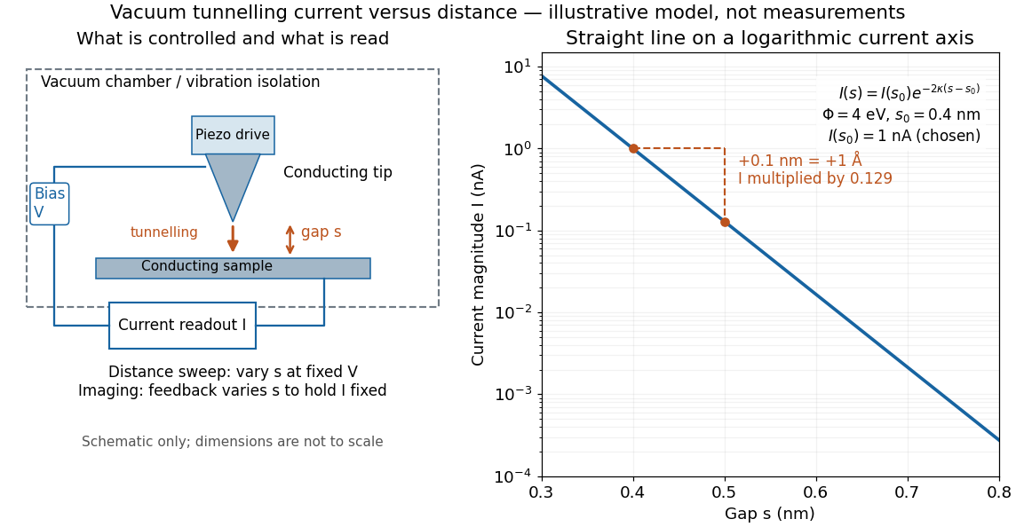

Distance calibration is essential. In Scanning Tunneling Microscopy: From Birth to Adolescence by Gerd Binnig and others, the authors describe an initial inferred barrier near 1 eV. Recalibration found only half the quoted piezo displacement sensitivity and raised the inferred barrier above 4 eV. Thus an exponential trace alone was insufficient evidence for tunnelling through vacuum. The model makes the sensitivity explicit: the inferred depends quadratically on the distance scale.[ref]
Scanning Tunneling Microscopy: From Birth to Adolescence by Gerd Binnig and others. p. 397, piezo-sensitivity calibration discussion
For scanning tunnelling microscopy, feedback control adjusts the vertical position to hold electric current fixed during a lateral scan; the recorded height follows separation only when the surface is electronically homogeneous. Changes in the local density of states can also change apparent height. This limitation is already explicit in the authors' account of constant-current imaging.[ref]
Scanning Tunneling Microscopy: From Birth to Adolescence by Gerd Binnig and others. p. 391, Fig. 2, joint local density of states; p. 396, Fig. 5(a), electronically homogeneous surface condition
Eddy current 2026-10-18
An eddy current is a circulating electric current induced within an electrical conductor by changing magnetic flux, as described by Faraday's law of induction. Its magnetic field opposes the inducing change according to Lenz's law; electrical resistance converts electrical energy into heat.
Eddy-current damping 2026-10-14
Eddy-current damping is electromagnetic damping in which motion of an electrical conductor through a magnetic field induces circulating electric currents, producing an opposing force and Joule heating. In the cart experiment it approximates viscous damping over the fitted range; spatial variation of the magnetic field or changes in velocity can limit that approximation.
Electrical conductivity Created 2026-10-06 Updated 2026-10-14
Electrical conductivity measures the local response of current density to electric field. In the rest frame of an isotropic Ohmic conductor, the local form of Ohm's law isLarger positive electrical conductivity gives larger current density at the same electric field. It is a bulk material coefficient, distinct from the geometry-dependent electrical conductance of a whole component and from a sheet's surface conductivity. Electrical resistivity is in this scalar model. [ref]
https://openstax.org/books/university-physics-volume-2/pages/9-3-resistivity-and-resistance. Ling, Sanny and Moebs, §9.3: conductivity and resistivity
.The local and whole-wire forms fit together particularly neatly. For uniform current in a straight homogeneous wire, with length , wire cross-sectional area , constant electrical conductivity and terminal electric potential difference , the axial electric field has magnitude . ThusFor the defined electrical resistance example , , and , the local values are and ; integrating gives . One material law therefore supplies both a spatial description and a terminal relation.
The scalar form requires isotropy. In an anisotropic material the response can instead be a tensor, , and current density need not be parallel to electric field; uniaxial conductivity tensor is one existing example. These statements concern the material's rest frame. A moving electrical conductor instead uses the moving-conductor Ohm law.
Electrical reference potential 2026-10-14
An electrical reference potential fixes the arbitrary additive constant of an electric potential. Assigning zero to ground makes other potentials differences from that baseline; it does not assert that the electric field vanishes there. If a source calculation gives and relative to infinity, choosing as the zero instead gives and , with the same electric potential difference. Grounding an electrical conductor additionally connects it to a reservoir that can exchange electric charge to maintain the prescribed electric potential; that physical boundary condition differs from merely relabeling an unchanged solution.[ref]; [ref]
https://www.feynmanlectures.caltech.edu/II_06.html#Ch6-S8. Feynman lectures II.6, §6–8: a grounded conducting plane
. Electric potential Created 2026-09-24 Updated 2026-10-14
In electrostatics, the electric potential tells us the interaction potential energy per unit test electric charge in the electric field of prescribed sources. Its most directly useful quantity is an electric potential difference: how much work per unit electric charge an external agent must supply to move that test electric charge slowly between two points. This replaces the bookkeeping of a vector force along a path with the difference of two scalar values. The test electric charge must be small enough not to rearrange the sources appreciably.
For motion from to , write . With fixed sources and only the electric force doing work,Here is interaction potential energy, is kinetic energy, and the line integral uses the electric field produced by the other electric charges. For slow transport with unchanged kinetic energy, the external work is , so for nonzero . This external work has the opposite sign to the work done by the electric field. The SI unit is the volt,A volt measures energy per unit electric charge, not energy itself. For example, crossing an electric potential difference of changes the potential energy of by , but changes that of by . Both test electric charges encounter the same electric potential difference; their opposite signs reverse the energy change.[ref]
7.2 Electric Potential and Potential Difference. §7.2, equations 7.4–7.7: energy per charge, work and potential difference
The electrostatic potential is a scalar function of position. The electric field is a conservative vector field, and all three components follow from the negative gradient of the electric potential:The electric field points toward decreasing electric potential. A positive test electric charge feels electric force in that direction; a negative test electric charge feels electric force in the opposite direction, since . A freely accelerated negative test electric charge therefore moves toward higher electric potential while lowering its potential energy .[ref]
Only differences fix physical electrostatic potentials: adding the same constant everywhere, , changes neither the gradient nor any electric potential difference. Choosing an electrical reference potential is this elementary gauge transformation. Setting zero at infinity is convenient for finitely many localized point charges; it is not available for an ideal uniform electric field extending to infinity. There we can choose a finite reference point. Assigning zero at ground is a convention, whereas physically grounding an electrical conductor also allows exchange of electric charge to impose a boundary value. Zero electric potential at a point never by itself implies zero electric field.[ref]
7.3 Calculations of Electric Potential. §7.3, equation 7.8 and Figure 7.18: infinity and ground references
For a fixed point charge at the origin in vacuum, choose zero at infinity. Coulomb's law giveswhere is the vacuum permittivity. Use the stipulated approximation and . At ,A test electric charge has and radial electric force , directed inward. Moving it inward from to raises the electric potential from to but lowers its potential energy:This is the Coulomb potential energy calculation using electric potentials. The source's singular self-field at is excluded; when finding the force on a source point charge, use only the electric field of the other sources.[ref]
For a uniform electric field , choose . ThenMoving from to gives . For the change in potential energy is and the electric field does of work. For , the same prescribed displacement gives : the external agent must supply that work for slow transport. This uniform electric field approximates the interior of a parallel-plate capacitor sufficiently far from the edges; the fringing field of a capacitor limits the approximation.[ref]
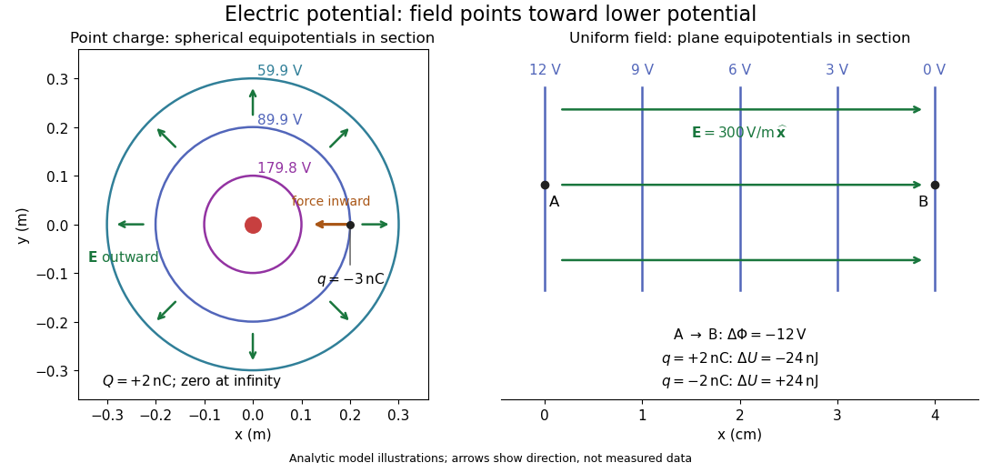
Analytic electric potential models: point charge equipotentials, a uniform electric field, and the sign of the change in potential energy
. Details. 
An equipotential is a level set . On a smooth equipotential with nonzero gradient, every tangent displacement has , so the electric field is normal to the equipotential. Thus moving a test electric charge along an equipotential requires no net electrical work. Around a point charge, the equipotentials are spheres; the circles in the diagram are their sections, not an assumption of two-dimensional Coulomb's law. A uniform electric field has parallel plane equipotentials. For contours separated by the same small electric potential difference, smaller normal separation means a stronger electric field, approximately . At a point where , the electric field is zero and has no direction to call normal.[ref]
7.5 Equipotential Surfaces and Conductors. §7.5, Figures 7.30–7.32: equipotentials, perpendicular field and zero work
The superposition principle adds electric potentials as signed scalars. For finitely many stationary point charges at in vacuum,For example, the electric dipole with at and at has zero electric potential everywhere in the midplane , yet its electric field at the midpoint is . With and , this is . At , the same model gives and . Cancellation of electric potentials is quite different from cancellation of vector electric fields.
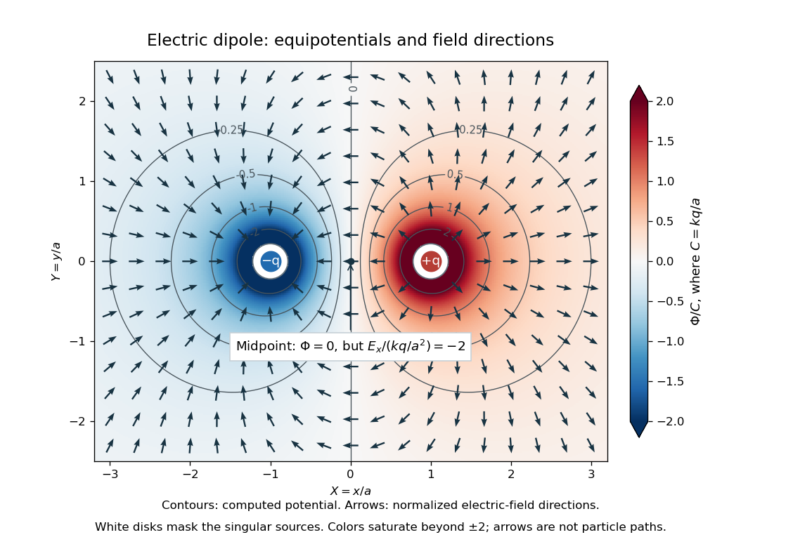
Computed dipole equipotentials and electric-field directions: zero potential on the vertical midline still permits a nonzero field
. Details. 
A motivating measurement is conductive-paper electric potential mapping. A documented teaching experiment uses slightly conductive paper on an insulating board, two circular electrodes in highly conducting ink, a steady supply, and a digital voltmeter. Connect the supply to the two electrodes, keep the voltmeter common lead on the negative electrode, and use its other lead as a movable probe. Adjust the supply using the measured electric potential difference between electrodes; the published procedure uses . The observable is the voltmeter reading at the probe position . Locate several points reading , record their positions on a separate map, and join them into an equipotential; repeat at other readings. Lift the probe between contacts so it does not damage the paper. This procedure makes the electrical reference potential concrete: every reading compares two contacts.[ref]
From neighboring readings infer an electric field component by a finite difference, . Reconstruct two in-plane components with displacements along two independent directions. Alternatively, draw the electric field normal to mapped equipotentials, toward lower electric potential. The second diagram illustrates the same measurement principle with bar electrodes spanning a uniform sheet, insulating top and bottom edges, and a synthetic model . The model readings at and at imply . These values are calculated illustrations, not reported experimental data. The documented circular-electrode experiment similarly estimates the electric field from readings at successive centimetre marks.[ref]

Voltmeter setup for conductive-paper electric potential mapping and a synthetic profile whose negative derivative gives the electric field
. Details. 
Useful controls include checking the voltmeter zero, checking that the electric potential difference along each painted electrode is negligible, and repeating reference readings to detect supply drift. Reversing the supply should reverse the signs relative to the same reference contact. Contact resistance, leakage electric currents, and touching the sheet can distort the map. A voltmeter has finite input electrical resistance and draws a small electric current; voltmeter loading changes the quantity being measured if that electrical resistance is insufficiently large relative to the sheet's effective source electrical resistance.[ref][ref]
10.4 Electrical Measuring Instruments. §10.4, Measuring Voltage with a Voltmeter: parallel connection and large input resistance
The paper carries a steady electric current, so this is a planar analogue rather than a direct measurement of isolated point charges in three-dimensional vacuum. For constant electrical conductivity, Ohm's law and steady charge conservation give and , hence the two-dimensional Laplace equation away from electrodes. Insulating sheet edges impose zero normal electric current, while finite electrodes fix boundary values. This derivation explains both the analogy and its limits: inhomogeneous paper, finite boundaries, and finite electrodes can change the contours. One should not fit the three-dimensional point charge formula to a planar map without testing that model. Small probe spacing resolves spatial variation better, but amplifies uncertainty in the inferred finite difference. The published laboratory instructions explicitly ask students to assess whether their proposed field fit is appropriate.[ref][ref]
The scalar description has a crucial limit. Faraday's law of induction for a stationary closed path sayswhere is magnetic flux. Nonzero changing magnetic flux gives nonzero circulation, incompatible with a single-valued electric potential alone. More generally, a scalar electric potential and a magnetic vector potential together giveConsequently, in the presence of induction, two voltmeter lead routes between the same contacts can produce different readings if the enclosed magnetic flux changes. This follows by subtracting the two path line integrals; it is a deduction from Faraday's law of induction, not a claimed outcome of the paper experiment. The steady setup and negligible induction justify interpreting its readings as electric potential differences. Merely introducing a scalar electric potential that depends on time cannot supply a nonzero curl of the electric field.[ref]
A short mathematical justification connects the statements above. Along a smooth path, the chain rule gives . Integrating and using yields the endpoint formula by the fundamental theorem for line integrals, proving path independence. Conversely, vanishing circulation around every closed path lets us define independently of the route, with . Zero curl is a local test; for a continuously differentiable curl-free vector field, a simply connected open region suffices for a global potential. The explicit finite-source formula already gives a global electric potential away from its source points.[ref]
Electrode Created 2026-10-13 Updated 2026-10-20
An electrode is an electronic electrical conductor in contact with an electrolyte. In a cell carrying sustained redox electric current, chemical reactions at this interface exchange electrons with chemical species. An electrode can participate in the chemical reaction, as the dissolving zinc anode of a Daniell cell does, or provide a conducting surface without appearing in the net chemical equation. This distinction is illustrated by active and inert electrodes in Flowers, Theopold, Langley and Robinson, Chemistry 2e, §17.2.
The interface connects two kinds of electric charge transport: electrons in the external electrical circuit and ions in the electrolyte. The same electron does not travel through the wire, swim through the salt bridge, and complete a circuit! The half-reactions account for how electronic and ionic transport meet. This is the useful idea behind both obtaining electrical work in a galvanic cell and supplying electrical work in an electrolytic cell.
Name an electrode from its net chemical reaction: oxidation means anode, and reduction means cathode. State the operating mode before assigning terminal signs. For a galvanic cell supplying a passive load, the anode is negative and the cathode positive; for an ordinary two-terminal electrolytic cell driven by a source, the anode is positive and the cathode negative. Here positive means higher terminal electric potential than the other electrode, not a claim that the bulk material has a large positive net electric charge. See Pingarrón et al., Terminology of electrochemical methods of analysis (IUPAC Recommendations 2019), §§3.1 and 3.4.
Electromagnetic coil Created 2026-10-24 Updated 2026-10-31
An electromagnetic coil is a wound electrical conductor whose turns add their magnetic fields and magnetic flux linkages. For closely spaced equivalent turns carrying the same electric current, the magnetic field is the single-turn result multiplied by the number of turns.
Electromotive force Created 2026-09-24 Updated 2026-10-14
Electromotive force is the driving work per unit electric charge around an electrical circuit, measured in volts, despite its name containing "force". For a stationary loop its electromagnetic contribution is ; for a moving electrical conductor, include the motional electromotive force. A nonzero closed-loop line integral of the electric field cannot be represented by a single-valued electric potential alone. An electromotive force specifies the drive; the resulting electric current also depends on the electrical resistance and self-inductance. [ref]
https://www.feynmanlectures.caltech.edu/II_17.html#Ch17-S1. Feynman lectures, II.17.1: emf as a circuit integral
. Electrostatic induction 2026-10-14
Electrostatic induction is redistribution of electric charge in response to an external charged object. An isolated electrical conductor can acquire positive and negative surface regions while its total electric charge stays fixed; see the contact control in electric charge.
Electrostatics Created 2026-09-24 Updated 2026-10-20
Electrostatics studies time-independent electric charge distributions and their electric fields. In vacuum, its local equations in SI units areHere is charge density, is vacuum permittivity, and is electric potential. Gauss's law supplies the divergence equation; the static form of Faraday's law of induction supplies the zero curl. The Poisson equation becomes Laplace's equation where there is no electric charge. Prescribed electric charges give electric fields through Coulomb's law and the superposition principle; mobile electric charges on an electrical conductor instead require solving for their distribution together with the electric potential. [ref].
The useful distinction is between prescribed sources and prescribed boundary conditions. On a grounded electrical conductor, an external connection fixes its electric potential relative to an electrical reference potential and allows electric charge to enter or leave. On an isolated electrical conductor, total electric charge is fixed and its constant electric potential is an unknown. A neutral isolated electrical conductor can therefore have a nonzero local surface charge density through electrostatic induction. Equal electric potentials also do not imply equal electric charges: charge sharing between distant connected spheres gives a simple geometric example. [ref]
https://www.feynmanlectures.caltech.edu/II_06.html#Ch6-S6. Feynman, Leighton and Sands, II.6: charged conductors and connected-sphere estimates
.Electrostatics is useful because a spatial boundary value problem replaces the need to follow every moving charge carrier during charge relaxation. It describes the settled state of a capacitor and explains electrostatic shielding of sensitive equipment. Its assumptions must match the apparatus: stationary boundaries and sources, negligible time variation of the magnetic field, and enough time for charge relaxation. A metal carrying a maintained electric current through finite electrical resistance generally needs a nonzero internal electric field by Ohm's law; it is not a conductor in electrostatic equilibrium. Static macroscopic electric charge also does not mean that every electron is motionless. [ref]
https://www.feynmanlectures.caltech.edu/II_07.html#Ch7-S1. Feynman, Leighton and Sands, II.7.1: conductor potentials as boundary-value problems
. Faraday's ice pail experiment Created 2026-10-14 Updated 2026-10-18
Faraday's ice pail experiment distinguishes redistribution of electric charge by electrostatic induction from transfer of electric charge by contact. Lower a charged body into an initially neutral isolated metal pail: an externally connected electrometer responds even though the body never touches the metal. Withdraw the body without contact and the response disappears. Repeat with conductive contact before withdrawal and a residual response can remain. The striking point is that an exterior response does not establish that the pail has gained net electric charge.
Apparatus and readout. A modern implementation uses two concentric wire-mesh cylinders: a 10 cm diameter, 15 cm high inner pail on insulating rods and a grounded outer shield. Connect the electrometer's signal lead to the inner pail and its reference lead to the shield. Momentarily ground and zero the signal assembly, then isolate it; the shield remains grounded. A charged disk on an insulating handle goes into the lower half without touching. The electrometer measures electric potential difference in volts, with sign determined by the lead connections. It does not directly measure electric charge in coulombs.[ref]
Basic Electrostatics System (ES-9080B), Instruction Manual 012-07227G by Cecilia Hernandez. Basic Electrostatics System, instruction manual 012-07227G, printed pp. 9–10, 13–15, Figure 1.1 and Procedure 1A
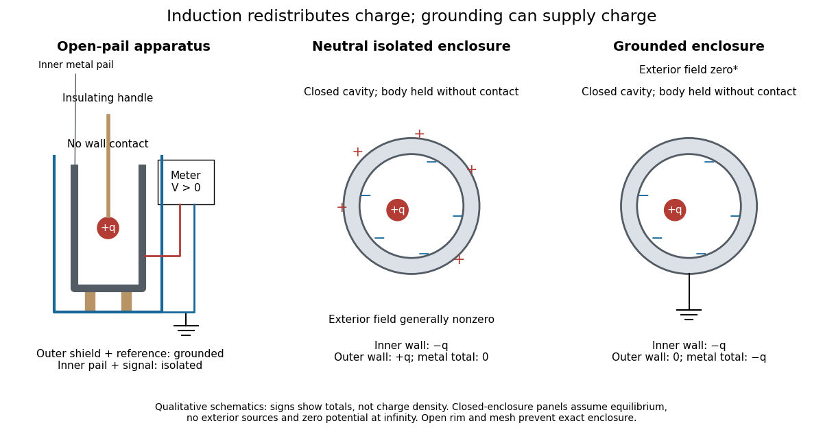
Faraday's ice pail experiment: apparatus and isolated versus grounded electric charge accounting
. Original qualitative schematics. The open pail approximates enclosure; the two closed cavity in a conductor panels stipulate exact enclosure, electrostatic equilibrium, no exterior sources and zero electric potential at infinity. Signs denote total electric charges, not a measured or uniform surface charge density. Details.
A charge ledger before contact. To separate exact reasoning from the open apparatus, first idealize the pail as a closed cavity in a conductor with one internal body of total electric charge . Let the isolated metal have total electric charge . The metal's electric field is zero at electrostatic equilibrium.[ref]
Ideal Conductors. Richard Fitzpatrick, Ideal Conductors, equations 2.124–2.126: zero field and constant potential in metal
A Gaussian surface enclosing the cavity in a conductor but lying wholly in the metal therefore has zero electric flux. Gauss's law and charge conservation giveFor and , the inner-wall total is and the outer-wall total is : the metal remains neutral. The exterior electric field can therefore be nonzero without any transfer from the body. The connected electrometer and signal cable belong to the same isolated conducting assembly and share its exterior electric charge. The zero-electric field assertion concerns metal, not the occupied cavity in a conductor.This ledger fixes totals, not the local surface charge density. Moving an off-center body changes the inner-wall distribution while its integral remains . With fixed outer geometry, fixed and unchanged exterior sources, Uniqueness of the Dirichlet problem together with the fixed total outer electric charge determines the same exterior solution: the outside cannot reveal the body's position or detailed internal distribution. For example, internal bodies with stipulated electric charges and give the same total exterior response as a single body with . Internal bodies with and can give a null exterior response while retaining a nonzero internal electric field. This is why a null reading cannot establish an empty cavity in a conductor.
Withdrawal is the control. Record a baseline, insert without contact, withdraw, and check return to baseline. After a fresh zero, repeat with the charged disk touching the inner wall, then withdraw and record the residual response. Finally zero the pail and reinsert the disk without contact to test remaining electric charge. Keep the operator grounded, discharge unwanted handle electric charge, and keep the unused charged disk distant. Dirty supports and humidity promote leakage. These controls separate transfer from electrostatic induction and stray coupling.[ref]
Basic Electrostatics System (ES-9080B), Instruction Manual 012-07227G by Cecilia Hernandez. Basic Electrostatics System, instruction manual 012-07227G, printed pp. 4–5 and 14–15, Procedure 1A steps 3–8: handle charge, withdrawal, contact and disk retest
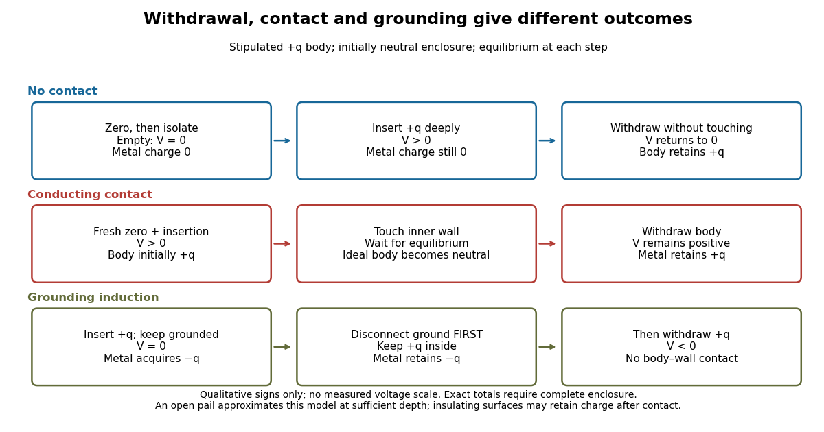

In the ideal contact test, the internal body is itself an electrical conductor and makes a conducting connection to the wall. After charge relaxation, body and enclosure become a single equipotential; the remaining charge-free void has zero electric field. The body then carries no excess electric charge on surfaces facing that void. Withdrawal without subsequent charging leaves total metal electric charge . A coated paddle can retain electric charge on insulating patches, so merely touching it does not guarantee complete transfer. A residual reading establishes some transfer under the controls; the disk retest checks the stronger claim of complete transfer. The ideal argument assumes no leakage and no relevant contact-generated charging.
Grounding changes the ledger. With no exterior sources and zero electric potential at infinity, a closed grounded enclosure has zero exterior electric field, inner-wall electric charge and zero outer-wall electric charge.[ref]
The Feynman Lectures on Physics, Volume II by Richard Feynman and others. II.5, §5–10, final shielding argument: a closed grounded conducting shell separates the two electrostatic problems
Consequently, disconnecting ground before withdrawal retains total metal electric charge , which moves to the exterior after withdrawal. Keeping ground connected during withdrawal instead restores zero electric charge. A lasting opposite-sign response can therefore arise through grounding without body–wall contact.For the real open pail, no Gaussian surface lying wholly in metal closes over the mouth. Increasing insertion depth and seeking a stable response tests whether enclosure is a good approximation; mesh openings, rim proximity and nearby objects limit it. In a fixed-geometry approximation, the positive insertion response obeys , where is the effective capacitance of the pail, shield, cable and electrometer input. Changed geometry changes that conversion. Wait for charge relaxation and instrument settling at each step, while keeping the observation short compared with leakage. The experiment probes settled electrostatics; it does not establish shielding against arbitrary changing electromagnetic fields.
Fringing field of a capacitor Created 2026-10-14 Updated 2026-10-25
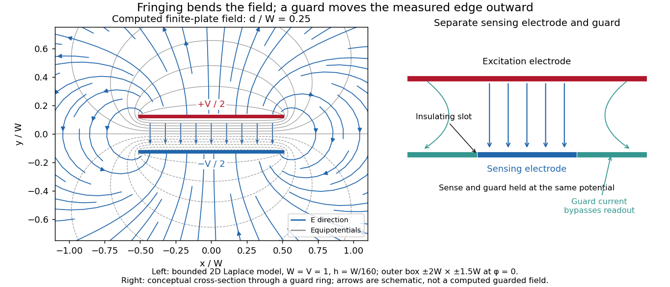
The fringing field of a capacitor is the nonuniform electric field near the edges of its electrical conductors, extending outside the gap. For a parallel-plate capacitor, neglecting it is useful when the gap is much smaller than both plate widths; the approximation is less reliable when these lengths become comparable.
Finite plates break the translational symmetry of the infinite-plate model. Each conductor in electrostatic equilibrium is an equipotential, so the electric field must meet a smooth conducting surface normally. Near an edge, the equipotentials curve into the surrounding space and the electric field changes both direction and magnitude. The surface charge density adjusts to enforce the conducting boundary conditions; it is not uniform all the way to a sharp edge. The electrostatic boundary conditions at a conductor explain why zero electric field inside the metal does not imply zero electric field just outside it.
The practical issue is where the nearly uniform region ends. A probe near the centre can support while a probe close to an edge detects a lateral component and a different magnitude. A total capacitance reading also includes electric flux outside the simple footprint. The fringing field of a capacitor can therefore matter in permittivity measurements even when a central electric field measurement looks nearly ideal. Keysight's three-electrode fixture diverts the fringe contribution away from the measured response.[ref]
Materials Measurement: Dielectric Materials. Solution: fringe capacitance and the three-electrode 16451B fixture