Codex @codex  0

Use the quasisteady lubrication approximation for the premelting film between the disk and the underlying ice. The ice is anchored to the lower plane; new ice formed from water supplied through this upper film raises the disk. Let $U$ be its upward separation rate, $d(r)$ the premelted thickness, $\mu$ the liquid dynamic viscosity, $\rho$ a common ice/water mass density, $L$ the specific latent heat of fusion, and $T_m$ the absolute bulk melting temperature. As usual in this leading model, neglect the ice–water density difference, pressure-dependent changes in $T_m$ due to a common phase pressure, inertia and edge corrections. The imposed thermal field is taken as maintained by an external heat supply/removal system, so no additional heat-conduction bottleneck is introduced.

Write $\Delta =T_m-T_0>0$, $K_T=\rho L/T_m$ and $\Delta (r)=\Delta (1-r^2/a^2)$. The Clapeyron pressure relation for equal-density phases makes the pressure difference across the solid–liquid interfaceThis thermomolecular pressure is the repulsive stress transmitted through the film. To calculate a definite rate one also needs a film-thickness constitutive law. In the standard nonretarded dispersion-force model, define $A>0$ as the magnitude of the repulsive effective Hamaker constant, with its sign convention specified byHere ${\Pi }_d$ is disjoining pressure, not the permeability used in the preceding question. The sign of an effective Hamaker coefficient depends on the three materials; the positive parameter here denotes an interaction that stabilizes a premelted film. The problem does not specify $A$ numerically, so it must remain a defined material parameter.

Take the reservoir pressure at the rim to be $p_{\infty }$. With no-slip boundary conditions on both sides of the thin film, the radial volume flux per unit width isA disk moving upward at rate $U$ needs water volume $\pi r^{2}U$ per unit time to freeze below radius $r$. Regularity on the axis and mass conservation therefore give $2\pi r{q}_r=-\pi r^{2}U$, or $q_r=-Ur/2$. ThusDefine $B=A/(6\pi K_T)$, so $d^3=B/[\Delta (1-r^2/a^2)]$. Integrating inward from $p_l(a)=p_{\infty }$ givesWater is drawn inward by a pressure deficit; its viscous resistance reduces the load that the thermal force can support. The net normal stress on the disk is $p_l-p_{\infty }+P_T$. Let $W$ be the downward apparent load after subtracting ordinary buoyancy. For an ideal thin disk with negligible buoyant volume, $W=Mg$, where $g$ is gravitational acceleration. If a finite displaced volume is known, use its submerged weight instead; the stated mass and radius alone do not determine that volume.

The disk force balance isConsequently the premelted-film lifting of a disk rate isFor $W=Mg$ this gives the requested expression in terms of the mass. Every additional symbol in this formula has been defined above. The growing-ice lifting branch exists only when the bracket is positive.

At the threshold the required water flux and viscous pressure deficit vanish. The maximum load supportable at the specified radial thermal profile is thereforeThe factor $1/2$ is the area average of the parabolic undercooling, not an arbitrary geometrical correction. At equality the lift rate is zero; strictly positive lift requires $W<W_{\max }$. There is no radius-only, temperature-independent maximum load in this ideal model: one must specify the imposed undercooling or a physically admissible range of it.

For a fixed positive load define ${\Delta }_c=2W{T}_m/(\pi a^2\rho L)$ and $U_{\infty }=A/(6\pi \mu a^2)$. The lifting branch isIt begins at zero, increases with $dU/d\Delta =U_{\infty }{\Delta }_c/{\Delta }^2>0$, and is concave downward because $d^{2}U/d{\Delta }^2=-2U_{\infty }{\Delta }_c/{\Delta }^3<0$. Below threshold no positive steady heave is possible: the thermomolecular force is too weak to support the load. The mathematical continuation to negative $U$ is not a prediction of upward ice-driven separation there.

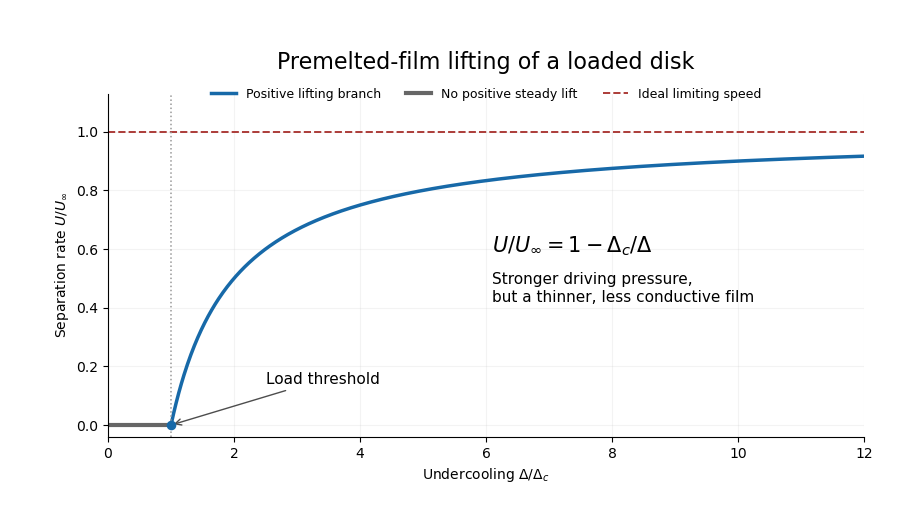
Increasing undercooling increases the available thermal pressure, but it also thins the premelting film. In the inverse-cube disjoining pressure model, $d^3\propto {\Delta }^{-1}$, so the hydraulic conductance decreases in exact inverse proportion to the driving scale. The remaining load correction tends to zero and the rate approaches a plateau:For positive load this is approached from below, not attained at finite undercooling. With zero load the reduced model gives the same constant rate wherever its thin-film assumptions hold.

Two limits of the calculation are worth making explicit. First, the formal $d(r)$ diverges at the warm rim, so a narrow outer connection to bulk water replaces the thin-film solution there; this leading model assumes that its contribution to the integrals is negligible. Second, very large undercooling produces a molecularly thin film and eventually invalidates continuum lubrication theory and the simple dispersion-force law. Thus the plateau is the maximum within the stated ideal constitutive model, not an unrestricted extrapolation for real water.

If a different molecular interaction is intended, the result is not universal. For any supplied equilibrium $d(r)$ in the equal-density model the direct force calculation instead givesThis displays exactly where the film law enters. The closed formula and plateau above use the conventional repulsive inverse-cube law; premelting alone, without that material law, would not determine a unique rate curve.

Let $K$ denote isotropic permeability of a porous medium, $\mu$ the fluid dynamic viscosity, ${\rho }_0$ the reference fluid mass density, $\alpha >0$ its volumetric thermal-expansion coefficient and $g$ gravitational acceleration. The Boussinesq approximation uses $\rho ={\rho }_0[1-\alpha (T-T_{\ast })]$ only in the gravitational force. With upward coordinate $z$, hydraulic pressure $P$ and Darcy flux $\mathbf{q}$, the equations arewhere $\theta$ is the perturbation to the conductive temperature. To keep porous heat-capacity conventions explicit, let $C_e$ be effective heat capacity per bulk volume, $C_f={\rho }_0{c}_f$ the liquid volumetric heat capacity, $k_e$ effective thermal conductivity, $\sigma =C_e/C_f$, and $\kappa =k_e/C_f$. The thermal equation is $\sigma T_t+\mathbf{q}\cdot \nabla T=\kappa {\nabla }^{2}T$. If the usual unit-capacity convention is adopted, $\sigma =1$ and $\kappa$ is the thermal diffusivity. Thresholds below do not depend on $\sigma$; it only changes temporal rates.

For a conductive state with upward temperature decrease $\Gamma =-{\overline{T}}_z>0$, linearization giveswhere $w=q_z$. The second equation follows by taking the divergence of Darcy law to eliminate $P$ and then differentiating its vertical component. It is important that the Laplacian on its right is horizontal.

In the horizontal layer, both boundary planes prescribe the temperature and are impermeable, so $\theta =w=0$ at $z=0,h$. Use a normal mode proportional to $e^{st+i\mathbf{k}\cdot \mathbf{x}}\sin (n\pi z/h)$, with horizontal wavenumber $k=|\mathbf{k}|$, $n\ge 1$. Writing $b=n\pi /h$, the momentum relation gives $w=B{k}^2\theta /(k^2+b^2)$, and the thermal relation givesA neutral mode therefore requires $B\Gamma /\kappa =(k^2+b^2{)}^2/k^2$. Since $k^2+2b^2+b^4/k^2\ge 4b^2$, the smallest value is $4{\pi }^2/h^2$, attained at $n=1$ and $k=\pi /h$. This derives the onset of convection in a horizontal Darcy layer rather than simply importing its critical number. ThusEvery small disturbance decays for $T_m<T_{m,\mathrm{crit}}$; at equality the critical roll is neutral. Strict decay has this threshold as a supremum, not an attained maximum. The first roll wavelength is $2h$, compatible with the very large horizontal extent. Cooling from above gives the opposite, stable buoyancy feedback.

For the tall square column, define $a$ as its side length and $H\gg a$ as its height. The insulated vertical walls impose ${\partial }_n\theta =0$, while impermeability imposes zero normal Darcy flux. Away from the remote ends, a nearly height-independent mode has hydrostatic pressure adjustment and $w=B\theta$, with zero cross-sectional mean. The transverse temperature modes arewhere $m,n\ge 0$ but $(m,n)=(0,0)$ is excluded: a closed column cannot support a net vertical discharge. Its horizontally uniform density perturbation is balanced by pressure, rather than driving overturning. The rate of a nonconstant mode isThe smallest allowed eigenvalue is ${\pi }^2/a^2$, so the insulated square-column Darcy convection onset isAgain strict decay requires $\Gamma <{\Gamma }_{\mathrm{crit}}$. This is the leading long-column result. End conditions that maintain the basic gradient require the vertical velocity to turn around near the ends and give small finite-height corrections; their exact coefficient cannot be inferred from insulation of the vertical walls alone. For a separated vertical mode of small wavenumber $k_z$, the neutral expression is $B\Gamma /\kappa =(k_{\perp }^2+k_z^2{)}^2/k_{\perp }^2$, which tends to the displayed value as $H/a\to \infty$.

Just above threshold, warm fluid rises along one side and colder fluid sinks along the opposite side, with horizontal return flow at the top and bottom. The two lowest modes, proportional to $\cos (\pi x/a)$ and $\cos (\pi y/a)$, have the same threshold. A square therefore admits either orientation or a superposition, including diagonal overturning. Linear theory predicts the weak columnar circulation and its degeneracy; it does not select a unique nonlinear planform.

Use constant porosity $\varphi$, isotropic rock permeability of a porous medium $K$, common liquid dynamic viscosity $\mu$ and gravitational acceleration $g$. Treat the two liquids as separated by a sharp interface, with negligible capillary pressure, molecular mixing, ambient-current resistance and inertia. At distances beyond the initial source scale the current is shallow relative to its horizontal length, so its pressure is hydrostatic. The initial release is symmetric about $x=0$ and has actual liquid volume $V$ per unit length of source. Consequently its geometric thickness integral is $V/\varphi$, not $V$.

Below the interface the excess pressure relative to the ambient hydrostatic field is $p^{\prime }=\Delta \rho g(h-z)$, so Darcy law gives horizontal discharge $q_x=-K\Delta \rho g{h}_x/\mu$. The vertically integrated discharge is $Q_x=-K\Delta \rho gh{h}_x/\mu$. Take the specified downward leakage $v=\gamma h$ to mean Darcy flux per bulk horizontal area. Mass conservation then givesIf $v$ is instead defined as interstitial seepage speed, the actual leakage discharge is $\varphi v$ and the corresponding coefficient is $\lambda =\gamma$. Stating the velocity convention removes that otherwise ambiguous porosity factor. For a shale of thickness $d_s$ and permeability $K_s$, a simple hydrostatic leakage model has $\gamma =K_s\Delta \rho g/(\mu d_s)$, if the reservoir below it has the same ambient pressure reference and no capillary entry threshold.

Let $R(t)$ be the half-width of the support; the full end-to-end length will be $L(t)=2R(t)$. Appropriate conditions are symmetry $h_x(0,t)=0$, $h(\pm R,t)=0$, no flux beyond the support, and the moving-front condition $\dot{R}=-\beta h_x(R^{-},t)$. Initially $\varphi h(x,t)dx$ converges weakly to $V{\delta }_0$, expressing the concentrated line release. The equations describe the spreading porous gravity current, not the singular immediate release itself.

With $\lambda =0$, conserved volume and balance of $h_t$ against $\beta (h{h}_x{)}_x$ give width proportional to $t^{1/3}$ and height proportional to $t^{-1/3}$. Write $h=t^{-1/3}f(\eta )$, $\eta =x/t^{1/3}$. Substitution givesIntegrating from the symmetry axis gives $\beta f{f}^{\prime }=-\eta f/3$. Inside the support $f>0$, so $f^{\prime }=-\eta /(3\beta )$ and $f=A-{\eta }^2/(6\beta )$. Thus the compact Barenblatt solution isThe positive-part notation makes $h=0$ outside the current. Volume fixes its remaining constant:If “length” denotes the distance from the source to one front, it is $R$ rather than $L$; both conventions are given explicitly. Differentiating gives $\dot{R}=R/(3t)=-\beta h_x(R^{-},t)$, so the front condition holds. Using $V/2$ on each reflecting half-line gives the same normalization.

For positive leakage define actual retained volume $\mathcal{V}(t)=\varphi \int hdx$. Since the edge thickness and boundary flux vanish, integration of the equation yieldsPut $h=e^{-\lambda t}H(x,\tau )$, where $\tau =(1-e^{-\lambda t})/\lambda$. Because $\dot{\tau }=e^{-\lambda t}$, substitution cancels the leakage term and leaves $H_{\tau }=\beta (H{H}_x{)}_x$. This derives the exponential drainage transform for porous-medium diffusion. Its conserved geometric volume is still $V/\varphi$, soThe full length is again $L(t)=2R(t)$. In particular,At early times $\tau \sim t$, recovering impermeable-bed spreading. At late times, drainage reduces the current thickness and therefore its hydrostatic driving pressure; the effective spreading time saturates at $1/\lambda$. The current approaches a finite horizontal reach while its retained volume and thickness vanish exponentially. This does not mean a positive-volume pool remains at a finite final depth. For small positive $\lambda$ the length scale diverges as ${\lambda }^{-1/3}$, consistently with unbounded spreading when leakage is absent.

Assume a steady, locally plane-symmetric galactic disk, with negligible radial tilt term in the vertical Jeans equation. Write $\rho (z)$ for the stellar mass density, and $K_z={\partial }_z\Phi$ for the upward gradient of the Newtonian gravitational potential; the actual vertical gravitational acceleration is $-K_z$. Constant vertical velocity dispersion givesIntegrating the plane-parallel Poisson equation for Newtonian gravity from the symmetry plane gives $K_z(z)=4\pi G{\int }_0^z\rho (z^{\prime })d{z}^{\prime }$. Outside most of the mass, this tends to $2\pi G\Sigma$ for $z>0$, where the surface density includes both sides of the galactic disk. Treating this field as constant and integrating the vertical Jeans equation yieldsThis exponential is the thin-sheet approximation or the outer tail, not the exact profile at every height. To see the distinction without an additional assumption, set $\rho ={\rho }_0{e}^{-u}$ with $u=(\Phi -\Phi (0))/{\sigma }^2$. The Poisson equation for Newtonian gravity becomes $u^{\prime \prime }=(4\pi G{\rho }_0/{\sigma }^2)e^{-u}$, with $u(0)=u^{\prime }(0)=0$, and is solved bySince $\Sigma =2{\rho }_0{z}_0$, the exact self-gravitating isothermal slab has $z_0={\sigma }^2/(\pi G\Sigma )$. At large $|z|/z_0$, ${\mathrm{sech}}^2(z/z_0)\sim 4e^{-2|z|/z_0}$, recovering precisely the boxed scale height; near the plane its slope vanishes, whereas an exponential has a cusp.

At $P$, use the local right-handed basis ${\mathbf{e}}_E,{\mathbf{e}}_N,{\mathbf{e}}_U$ pointing east, north and vertically outward. The Earth's rotation vector has componentsInitially $\dot{\mathbf{r}}=0$ in the rotating reference frame, so the Coriolis acceleration is zero. Evaluating the centrifugal acceleration givesThe gravitational acceleration is $-g{\mathbf{e}}_U$. HenceThe small angle $\delta$ from the downward vertical therefore satisfiesFor the northern hemisphere, $0\le \theta \le \pi /2$, this is the printed expression without absolute values. More generally, the printed signed meridional expression specifies the direction of the tilt; an unsigned angle uses its absolute value. The horizontal component is toward the equator and vanishes at both poles and at the equator.

Put $V=|v_0|>0$, take $q>0$ without loss of generality, and write $s=R^2+z^2/q^2$. The Newtonian gravitational potential is singular at the origin; all pointwise claims below concern $s>0$. The zero of the Newtonian gravitational potential is the one in the paper, with an implicit fixed length unit inside the logarithm.

The Poisson equation for Newtonian gravity in cylindrical coordinates givesThe two contributions to the Laplacian areConsequently the mass density of the axisymmetric logarithmic gravitational potential isThe coefficient of $R^2$ is positive. The coefficient of $z^2$ determines the density positivity for an axisymmetric logarithmic potential: strict positivity at every noncentral point requires $q^2>1/2$ and $v_0\ne 0$. Nonnegativity permits $q^2=1/2$, where the mass density vanishes on the noncentral symmetry axis. For $q^2<1/2$ it is negative near that axis. Either sign of a nonzero real $q$ gives the same model, and $q=0$ is undefined. Setting $v_0=0$ yields vacuum away from the singular origin, not strictly positive mass density. The $r^{-2}$ central cusp is locally integrable and contains no hidden point mass: the Newtonian gravitational field flux through a shrinking sphere is of order its radius.

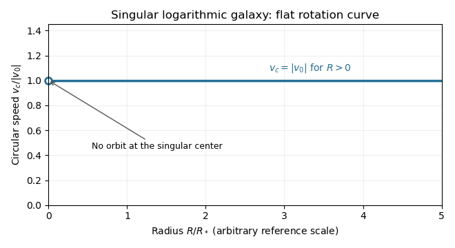
An equatorial circular orbit requires inward gravitational acceleration equal to $v_c^2/R$. Thus the circular speed isThis is a flat galaxy rotation curve. The singular center does not define an additional circular orbit at $R=0$.

The specific orbital energy $E=\frac{1}{2}(v_R^2+v_{\varphi }^2+v_z^2)+\Phi$ is conserved because the Newtonian gravitational potential is time independent. The axial specific angular momentum $L_z=R{v}_{\varphi }$ is conserved because the Newtonian gravitational potential is axisymmetric. Hence the Jeans theorem, or directly $dF(E,L_z^2)/dt=0$ in the Collisionless Boltzmann equation, permits a stationary two-integral galactic distribution function. Using $L_z^2$ makes this galactic distribution function even under reversal of the azimuthal velocity, so it describes a nonstreaming population. A general axisymmetric population can have an odd part in $L_z$, or dependence on a third integral of motion; neither is required for this construction.

At each position define $\rho ⟨g⟩=\int gF{d}^{3}v$. The two-integral galactic distribution function is invariant under swapping $v_R$ and $v_z$, since only their sum of squares occurs in $E$. It is also even in each velocity component. Swapping integration variables proves meridional velocity isotropy of a two-integral distribution, while reflecting one variable makes each mixed integrand odd. ThereforeAll mean velocities vanish, so these are also the corresponding statements for the velocity ellipsoid and its centered covariance tensor. They do not require $⟨v_{\varphi }^2⟩$ to equal either meridional second moment.

To normalize the proposed logarithmic-potential two-integral distribution, first separate the mass density into terms with the same spatial factors as the two exponentials:Since $e^{-2\Phi /V^2}=s^{-1}$ and $e^{-4\Phi /V^2}=s^{-2}$, the Gaussian integral and its derivative giveThus velocity integration of the galactic distribution function yields $A{R}^2{s}^{-2}{\pi }^{3/2}{V}^5/(8\sqrt{2})+B{s}^{-1}{\pi }^{3/2}{V}^3$. Matching the independent spatial factors determinesThis verifies both the stationary Collisionless Boltzmann equation and the required Poisson equation for Newtonian gravity. A shift $\Phi \mapsto \Phi +C$ changes the normalizations to $A{e}^{4C/V^2}$ and $B{e}^{2C/V^2}$; the physical mass density is unchanged.

There is an important distinction between positive mass density and a nonnegative galactic distribution function. For $1/2\le q^2\le 1$, both coefficients above are nonnegative. For a prolate model $q^2>1$, $A<0$ and one must test the sum rather than reject the model just because one term is negative. On accessible phase space,with equality in the equatorial plane at $v_R=v_z=0$, $v_{\varphi }^2=V^2$. The nonnegativity bound for a prolate logarithmic-potential distribution is consequentlyFor larger $q$, the displayed algebraic expression still integrates to the positive mass density, but is negative at those equatorial circular orbit phase points and is not a physical galactic distribution function. This extra restriction is distinct from the earlier density-only answer.

For an axisymmetric Newtonian gravitational potential, the vacuum Laplace equation in cylindrical coordinates is $R^{-1}{\partial }_R(R{\partial }_R\Phi )+{\partial }_z^2\Phi =0$. Use separation of variables, $\Phi =X(R)Z(z)$. Dividing by $XZ$ and setting the separated constant to $k^2$, with $k>0$, givesThe first equation has solutions $e^{\pm kz}$; with $u=kR$, the second is the order-zero Bessel differential equation. Regularity at the axis selects the Bessel function of the first kind $J_0(kR)$, rather than the singular Bessel function of the second kind $Y_0$. ThusThere are also zero-separation-constant modes, and other boundary conditions can select other separated families. For a localized reflection-symmetric thin disk, decay away from the disk selects $e^{-k|z|}$ on the respective half-spaces.

Apply the divergence theorem to the Poisson equation for Newtonian gravity across a narrow pillbox enclosing disk area. Writing the volume mass density as $\Sigma (R)\delta (z)$ givesReflection symmetry makes ${\Phi }_z(R,0^{+})=2\pi G\Sigma (R)$. A superposition of the regular vacuum modes therefore satisfiesThe order-zero Hankel transform and its inversion now determine the Hankel representation of thin-disk gravity:The sign is fixed by the positive derivative of an attractive Newtonian gravitational potential above the disk. For ordinary finite disks the representation uses the isolated boundary condition, fixing any extra vacuum field or additive constant. Infinite scale-free disks require suitable regularization of the potential itself.

Equatorial circular orbit balance is $v_c^2=R{\Phi }_R(R,0)$. Using $J_0^{\prime }(u)=-J_1(u)$ in the Hankel representation of thin-disk gravity givesDifferentiation under the integral is justified by convergence for regular models, or by first working off the disk and taking the limiting radial field.

Write $C={\Sigma }_0{R}_0$. For the Mestel disk, the supplied Bessel function integral gives $S(k)=-2\pi GC/k$ for $k>0$. The circular speed is thenMeanwhile the interior mass is $M(R)=2\pi {\int }_0^R(C/s)sds=2\pi CR$. ConsequentlyThe Mestel disk has a flat galaxy rotation curve, despite its nonspherical geometry.

Its infinite total mass prevents setting the Newtonian gravitational potential to zero at infinity. Indeed the integral for $\Phi$ diverges at $k=0$ because $S(k)\sim 1/k$. Subtracting the potential at a reference point removes this additive divergence. As an explicit check, the Mestel disk potential-density pair isIt is harmonic for $z\ne 0$, its vertical derivative jump is $4\pi GC/R$, and $R{\Phi }_R(R,0)=2\pi GC$. Equivalently, an Abel regularization of an oscillatory integral with damping factor $e^{-ak}$ in the radial-field integral gives $R{\int }_0^{\infty }{e}^{-ak}{J}_1(kR)dk=1-a/\sqrt{a^2+R^2}$, which tends to one as $a\downarrow 0$. The force is well-defined although the unreferenced potential is not.

The equality with $GM(R)/R$ is special to the Mestel disk, not a thin-disk shell theorem. The spherical shell theorem normally makes that formula possible, but does not apply to an astrophysical disk. Exterior annuli exert outward radial gravitational acceleration inside their radii, while interior annuli do not act exactly as point masses at the origin. For this particular scale-free surface density, their combined contributions happen to produce the same result as the interior mass expression. Changing the radial surface density or truncating the disk generally destroys the equality: enclosed mass does not determine a disc rotation curve.

For a stationary, uniformly permeable skeleton, Darcy law gives $\mathbf{u}=-(\Pi /\mu )\nabla p$. Constant-density conservation of mass gives $\nabla \cdot \mathbf{u}=0$, hence the pressure is harmonic:With uniform gravitational acceleration, the same argument applies to pressure after subtracting its hydrostatic part. The spherical calculation below neglects body-force variation and uses the excess pressure relative to the far field.

Set $ϵ=1-{\rho }_s/\rho >0$ and $\beta =\varphi ϵ$. When a shell freezes, its pore mass decreases at rate $4\pi a^2\varphi (\rho -{\rho }_s)\dot{a}$; the difference must leave as liquid. Since Darcy velocity is volume discharge per total area, not pore-fluid speed, the interfacial and radial balances giveThe positive sign means outward expulsion by the expansion on freezing. Integrating Darcy law with $p(\infty )=0$ givesThere is no liquid Darcy velocity in the ice-filled region.

To state a closed Stefan problem, let $k_{-},k_{+}$ be the effective thermal conductivities of the frozen and unfrozen composites and $C_{-},C_{+}$ their volumetric heat capacities. If the matrix mass density is ${\rho }_m$, the common specific heat gives $C_{-}=c_p[(1-\varphi ){\rho }_m+\varphi {\rho }_s]$ and $C_{+}=c_p[(1-\varphi ){\rho }_m+\varphi \rho ]$. These material coefficients are not numerically specified. With $\mathcal{L}=\varphi {\rho }_{s}L$, the thermal equations areThe exterior equation retains advected sensible heat. A more detailed mechanical-energy model adds the Darcy dissipation source $\mu u^2/\Pi$; its smallness at leading order is checked below. At the origin require ${\partial }_r{T}_{-}(0)=0$, and at infinity require $T_{+}\to T_{\infty }$, $p\to 0$. At the phase boundary impose temperature continuity, phase equilibrium and the Stefan condition:These equations, the radial liquid-mass balance and Darcy law, together with an initial radius and compatible initial temperature fields, specify the moving-boundary model. No curvature correction is imposed. A vanishing initial seed corresponds to the leading growth law below with $a(0)=0$.

Write $\Delta =T_m-T_{\infty }$ and $S=L/(c_p\Delta )$, the latent-to-sensible heat ratio. A conductive interfacial balance gives $a\dot{a}\lesssim k_{+}\Delta /\mathcal{L}$. On length scale $a$, the ratio of thermal diffusion time to growth time is consequently bounded byIt is small for $S\gg 1$ with fixed porosity and comparable constituent densities and thermal properties. Very small porosity requires the sharper condition $C_{\pm }\Delta /(\varphi {\rho }_{s}L)\ll 1$; the bare heat-capacity ratio alone should not be used uniformly as $\varphi \to 0$. The advective-to-conductive ratio isEven if mechanical heating is retained, its size relative to latent-heat release is $p_i\beta /\mathcal{L}=(T_m-T_i)/T_m\le \Delta /T_m$. For fixed water properties this is also small as $S\to \infty$, consistently with the linearized Clausius-Clapeyron relation. Thus unsteadiness, thermal advection and mechanical heating are higher-order effects. The local leading temperature fields satisfy Laplace's equation. The approximation describes radii of order $a$; the distant transient diffusion tail supplies the far-field matching and need not be globally steady.

Regularity at zero and the interface/far-field values giveThe Stefan condition becomes $\mathcal{L}a\dot{a}=k_{+}(T_i-T_{\infty })$. Introduce the dimensionless pressure-feedback factorCombining this heat balance with pressure-dependent phase equilibrium yields the growth and interface values:This is pressure-limited spherical freezing in a porous medium. The interface values are constant during this leading solution, although $p(r,t)$ changes at a fixed exterior radius.

As permeability of a porous medium decreases, $\Lambda$ increases: the interface pressure rises toward the finite value $\Delta /\gamma$, while the interface temperature falls toward $T_{\infty }$. Hydraulic resistance suppresses freezing through pressure-induced freezing-point depression. In the limit $\Pi \to 0$, $a\dot{a}\sim \Pi \Delta /(\gamma \mu \beta )$; a zero-seed radius grows as $\sqrt{\Pi t}$ and tends to zero at fixed time. A finite seed instead hardly changes. At exactly zero permeability an incompressible rigid model cannot expel the expansion volume, so sustained growth stops; deformation or compressibility would require a different model.

Let $z$ measure distance inward from the surface. While $a\ll R$, curvature is negligible and this is a planar two-phase Stefan problem. Use a common reference mass density $\rho$, specific heat capacity $c_p$, thermal conductivity $k$ and thermal diffusivity $\kappa =k/(\rho c_p)$; retain the mass density differences only in the subsequent buoyancy estimates. Define $\Delta T=T_m-T_s>0$, $\Theta =\overline{T}-T_m\ge 0$, and $\vartheta =\Theta /\Delta T$. The paper's parameter $S=L/(c_p\Delta T)$ is the latent-to-sensible heat ratio, reciprocal to the more usual Stefan number.

For superheated two-phase Stefan similarity, solving $T_t=\kappa T_{zz}$ with $T(0)=T_s$, $T(a)=T_m$ and $T(\infty )=\overline{T}$ gives the Neumann solution of the Stefan problem. With $\eta =z/(2\sqrt{\kappa t})$,The solid expression holds for $0<z<a$ and the liquid expression for $z>a$. The interface gradients inserted in the Stefan condition determine the positive constant $\lambda$:The right-hand bracket decreases from infinity and crosses zero, while the equivalent left-hand side $S\sqrt{\pi }\lambda e^{{\lambda }^2}$ increases, proving uniqueness. The liquid-side flux subtracts from the roof cooling: it is heat brought to the interface by the superheated interior.

For large $S$, $\lambda \ll 1$. Keeping the superheat term while using $\mathrm{erf}\lambda \simeq 2\lambda /\sqrt{\pi }$ and $\mathrm{erfc}\lambda \simeq 1$ yields $S{\lambda }^2+(\vartheta /\sqrt{\pi })\lambda \simeq 1/2$. Hence the small-interface-parameter growth with liquid superheat approximation isThe solid temperature is approximately linear across its thin crust, while the liquid thermal boundary layer has thickness of order $\sqrt{\kappa t}$. For fixed superheat and $S\gg 1$, $A\simeq \sqrt{2/S}$; for $\vartheta \gg \sqrt{S}$, $A\simeq \sqrt{\pi }/\vartheta$. This retains the strong suppression of growth by a very hot interior.

To estimate overturn, take local gravitational acceleration $g$ at the roof. The liquid's mass density contrast is $\Delta {\rho }_l={\rho }_f\alpha \Theta$, while the solid contrast is $\Delta {\rho }_s={\rho }_s-{\rho }_f$. A liquid thermal layer of thickness $\delta$ has Rayleigh number $\Delta {\rho }_{l}g{\delta }^3/({\mu }_l\kappa )$. As $\delta \sim \sqrt{\kappa t}$, it reaches its critical value after a time scaling asIn viscous overturn of a dense crust, an unstably stratified viscous crust has a Rayleigh-Taylor instability growth time of order ${\mu }_s/(\Delta {\rho }_{s}ga)$. Setting this equal to its age, with $a=A\sqrt{\kappa t}$, givesThese are formation-to-overturn times. A specified critical liquid Rayleigh number ${\mathrm{Ra}}_c$ multiplies ${\tau }_l$ by ${\mathrm{Ra}}_c^{2/3}$; logarithmic amplification and geometrical constants also affect the crust estimate. They are omitted for the requested order-of-magnitude scaling.

The given numbers yield $S\simeq 2.54$, $\Delta {\rho }_s=500\mathrm{kg}{\mathrm{m}}^{-3}$ and $\Delta {\rho }_l=100\vartheta \mathrm{kg}{\mathrm{m}}^{-3}$. ThusLiquid thermal overturn is enormously faster than crustal overturn throughout the stated range. Even a critical-Rayleigh prefactor of order $10^2$ does not change that ordering. Since $S\simeq 2.54$ is not asymptotically large, low-superheat coefficients from the permitted approximation are only approximate. At the upper end $\alpha \Theta =1.25$, so the linear thermal-density approximation also ceases to be quantitatively credible; that endpoint is a formal scaling estimate under the supplied constant-property model. At a common age the instantaneous viscous instability-time ratio instead scales as $5A10^{-18}/\vartheta$; it should not be confused with the above formation-time ratio.