We prove the equivalence by a cycle of implications. First assume closedness and boundedness. Given a sequence in , boundedness puts each coordinate in a fixed closed bounded real interval. Apply the one-dimensional Bolzano-Weierstrass theorem to its first coordinate to extract a convergent subsequence, then apply it to the second coordinate of that subsequence, and continue through the finitely many coordinates. The final subsequence converges coordinatewise to some . It also converges in the Euclidean norm, since the sum of the squares of its finitely many coordinate differences tends to zero. Since is a closed set, this limit belongs to . Thus closedness and boundedness imply the required subsequence property. No higher-dimensional compactness theorem has been assumed.
Assume the subsequence property, and let be a continuous function. If were unbounded, for each positive integer we could choose with . There is a subsequence with . By continuity, , so that real sequence is bounded. But , a contradiction. Hence every continuous real-valued function on is bounded. This is the bounded-function consequence of sequential compactness.
Assume every continuous function is bounded. The Euclidean norm function is continuous, so its boundedness proves that is a bounded set.
If were not a closed set, there would be . Choose with . The function is continuous everywhere on , because its denominator is nonzero there. Yet , contradicting the hypothesis. Thus is closed. Together with the two previous implications this proves all three conditions are equivalent. The empty set satisfies all three conditions trivially. This is the Euclidean case of the bounded-continuous-function characterization of compact metric spaces.
For positive differentiable speed and a smooth ray written as a graph , the Fermat principle minimizes travel timeA variation vanishing at the endpoints gives the Euler-Lagrange equation for . Its derivatives are and . Thusand multiplying by givesThe displayed differential equation requires differentiability, beyond mere continuity of . For constant positive speed it reduces to , so rays are straight lines; a straight segment minimizes travel time because it has the shortest Euclidean length.
For in the positive-height region, the Beltrami identity gives . Hence , whose nonvertical solutions are . Formally imposing the given boundary points fixes , , and gives the ray in a linear-speed mediumIt is the upper semicircle of diameter one, with vertical limiting tangents at its endpoints.
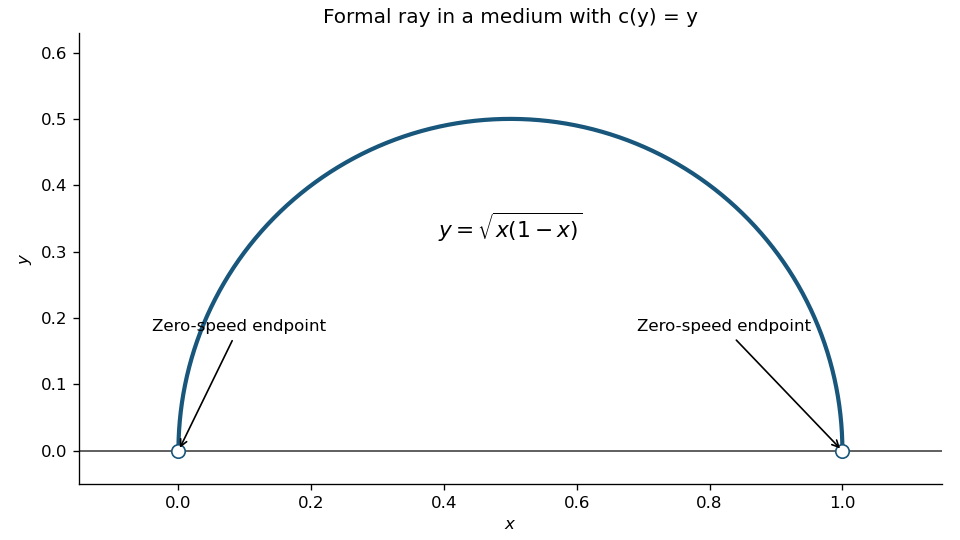
There is a necessary endpoint qualification. The speed is zero at the two stated endpoints. For any rectifiable path entering positive height, , and its travel time diverges logarithmically on leaving or approaching height zero. Thus the semicircle is the formal interior ray, but there is no finite-time minimizer between the zero-speed endpoints. For endpoints at height the circular ray has radius and finite travel time , which tends to infinity as . This explains the intended semicircle as a limiting hyperbolic geodesic, without asserting finite travel time where .
Put , so . The ordinary least squares criterion is . Setting both partial derivatives to zero gives and . Therefore, provided , the centred simple linear regression estimators areThe Hessian of is , which is positive definite, so this stationary point is the unique minimum. From the mean-zero errors, both estimators are unbiased; independence and common error variance give , , and zero covariance. Normality is not needed for this derivation. If all coincide, the slope is not identifiable and only the intercept is determined.
Using the PDF data gives , , and . In particular, the fourth cost is 37 in the PDF; the TeX's 75 is a transcription error and would contradict the supplied covariance sum. The fitted simple linear regression isHere the centred intercept estimate is 42.4; an intercept at would instead be . For eight units the predicted unit cost is
Use the Poincaré half-plane model, with metric . Its hyperbolic lines are vertical lines and semicircles centred on the real boundary, hence orthogonal to that boundary. Each has two ideal endpoints in . Distinct parallel hyperbolic lines are disjoint inside and share one ideal endpoint; distinct ultraparallel hyperbolic lines are disjoint and share none. Intersecting lines are neither. Because the metric is conformal to the Euclidean metric, the two notions of angle agree.
Apply a hyperbolic isometry taking one line to the imaginary axis, whose ideal endpoints are . If the other line is ultraparallel, its endpoints are two finite nonzero real numbers of the same sign. Reflect if necessary to write them as . Then is the semicircle with centre and radius .
Every hyperbolic line perpendicular to the imaginary axis must be a semicircle centred at zero: at the intersection its tangent has to be horizontal, forcing its real centre to coincide with zero. Let its radius be . Orthogonality to the circle representing requires , since the radii to the intersection form a right triangle. ConsequentlyThis has exactly one positive solution. The circles intersect above the real axis: . Hence the required common perpendicular of ultraparallel hyperbolic lines exists and is unique.
Conversely, if intersects the imaginary axis, its endpoints straddle zero and the same equation would require , which is impossible. If has endpoint zero, it gives , not a line. If its shared endpoint is infinity, is another vertical line; no circle centred at zero meets a distinct vertical line with horizontal tangent. Thus parallel lines have no common perpendicular either. These cases exhaust distinct lines, proving a unique common perpendicular exists exactly for ultraparallel lines.
Define the linear map by the two prescribed left-hand sides. Then , so it is a vector subspace: it contains zero, and linear combinations of vectors with zero image still have zero image.
Subtract the first equation from the second to obtain . The first equation then gives . ConsequentlyEach of the three displayed vectors satisfies both equations, and the decomposition proves they span . If their linear combination is zero, its third, fourth and fifth coordinates respectively force all three coefficients to vanish. They are therefore linearly independent, giving the basis
Follow a fluid particle released at time , and use for its running time. Its pathline satisfies , and , with zero position at . Hence , , andAt observation time , set . Substitution gives the streaklineThe curve is parameterized by release times . If release starts at time zero, only is occupied. This is a streakline, the positions of different particles released at one fixed point, rather than an instantaneous streamline of this unsteady flow.
Since and are harmonic conjugates, is a holomorphic function on , with and . The entire function can be composed with . Its value isBy the complex chain rule the composition is holomorphic on , so its real and imaginary parts obey the Cauchy-Riemann equations. They are harmonic as well: differentiating those equations gives and likewise . Hence are a pair of harmonic conjugates on . No simple-connectivity assumption is needed because the conjugate pair is already supplied globally. The PDF has in both expressions; the differing TeX exponents are transcription defects.
Nondegeneracy of means both radicals are zero: if for every , then , and the analogous implication holds in the other variable. Define linear maps and by and . Both are injective. Finite dimensionality gives and , so they are isomorphisms.
Similarly define and , which are linear by bilinearity. SetThen and are linear endomorphisms of and , respectively, and their definitions give for every pair. These dual isomorphisms induced by a nondegenerate pairing also prove uniqueness. No symmetry of , and no identification of the two vector spaces, is required.
Interpret the box as an infinite square well, with zero potential on and impenetrable walls. The wavefunction vanishes at both walls. The time-independent Schrödinger equation inside is . Multiplying by and integration by parts shows for any nonzero state with the wall conditions.
For , put . The condition at zero gives , and the condition at requires . The zero value of gives only the zero wavefunction, so the allowed energy eigenvalues areThe corresponding normalized energy eigenstates are . Each level is nondegenerate in this one-dimensional problem. A nonzero constant interior potential would add that constant to all energies.
A metric space is a set with a nonnegative symmetric distance , zero exactly for equal points, satisfying . A Cauchy sequence is a sequence for which, given any , there is such that whenever .
For a pseudometric, zero distance defines an equivalence relation. Reflexivity and symmetry are immediate; transitivity follows from when both terms vanish. Define . If and , the triangle inequality gives and its reversed version gives equality. Thus the definition is independent of representatives. The nonnegative, symmetric and triangle properties descend, while zero distance means precisely that the two classes are equal. It is therefore a metric quotient of a pseudometric.
Now take two Cauchy sequences in the original metric space. Two applications of the triangle inequality giveThe right-hand side is arbitrarily small when both indices are large, so is a real Cauchy sequence and has a finite real limit. Consequentlyis well defined. Nonnegativity, symmetry and zero self-distance follow by passing to the limit in the corresponding properties of . Passing to the limit in gives its triangle inequality. Thus is a pseudometric on , and the preceding quotient construction makes a metric space.
Map to the class of its constant sequence. The distance between two such classes is , so this is an injective isometric embedding. It is surjective exactly when every Cauchy sequence is equivalent to a constant sequence , that is, when for some . This is precisely completeness. HenceThe quotient is the Cauchy-sequence construction of a metric completion; the conclusion requires no assumption that is compact.
Away from the source point, the Green function obeys the homogeneous equation and must satisfy the appropriate endpoint condition. Thus it has the form to the left of and to the right. It must be continuous at : otherwise its second distributional derivative would contain an unwanted derivative of a Dirac delta. Integrating across gives the jump condition .
The left and right homogeneous solutions , have constant WronskianThis is nonzero for real noninteger . Dividing the product of the left and right solutions by that Wronskian therefore gives the Dirichlet Helmholtz Green function on an intervalThe formula vanishes at both endpoints, is continuous at the source and has derivative jump one, verifying all distributional and boundary conditions. A difference of two such Green functions would be a homogeneous Dirichlet solution; it vanishes because , proving uniqueness. Although zero is excluded by the stated noninteger condition, the removable limit is .
First use a homogeneous solution to meet the nonzero endpoint values:It satisfies , and . The Green-function representation then givesApplying the differential operator to the integral gives by the defining Dirac delta property of , and that integral vanishes at the endpoints. For continuous this is a classical solution; integrable also gives the corresponding weak solution. The same nonresonant homogeneous argument as in part (a) proves uniqueness.
Assume the two normal samples are independent. Write , , and let denote their residual sums of squares about the respective sample means. The joint likelihood function, apart from its constant factor, iswhere , . For every fixed variance pair the means maximize this likelihood at , because , and likewise for .
Under equal variances, differentiate the profiled log-likelihood to obtain . Without the order constraint, the separate variance maxima are , . If they lie in the alternative. If their order is reversed, maximizing over puts the optimum on the equal-variance boundary. These assertions also follow by strict concavity in the precisions .
Thus the one-sided likelihood-ratio test for two normal variances uses the quotient of the null maximum to the maximum over null and ordered alternative:To identify the rejection direction, put . Up to constants, . Its derivative is , negative on the ordered branch . Hence small likelihood ratios mean a large sample variance ratio.
The null law must account for estimating both means. By Cochran's theorem, and are independent random variables with chi-squared distributions of 5 and 20 degrees of freedom. Consequently the exact null statistic isIt is an increasing multiple of , so an upper-tail critical region is the likelihood-ratio rejection region. The observed statistic is . The supplied 95th percentile is 2.71, soThe F-distribution degrees of freedom are , not , although the variance maximum-likelihood estimates themselves have denominators .
The Poincaré half-plane model has Riemannian metric . Every Möbius transformation preserving this half-plane can be represented as with real coefficients and . Direct calculation givesTherefore , proving it is an isometry.
The imaginary axis is a hyperbolic geodesic. Its distance from to is . This is also the minimum over all paths, since path length is at least . The two vertical points at distance from are and . Reflection in the imaginary axis preserves the hyperbolic circle and its centre. Since it is assumed to be a Euclidean circle, its Euclidean centre lies on that axis and its two vertical intersections determine the Euclidean centre and radius:This proves the hyperbolic circle in the upper half-plane formula for the specified centre.
For the horizontal-distance calculation, the geodesic joining to is the semicircle of centre and radius . Parameterize it as . Its metric length is . If the right endpoint angle is , then , , and the other endpoint angle is . HenceThe equality of horizontal hyperbolic and Euclidean distances therefore requiresLet . The derivative of has the sign of . This quantity vanishes at zero and has derivative , so the height function is strictly decreasing. Its limits are one at and zero at . Continuity and the intermediate value theorem prove that each has exactly one positive matching separation .
Choose a basis for . Extend it to a basis of , and separately to a basis of . The combined list spans .
To prove linear independence, suppose a linear combination of the combined list is zero. Then the combination of the lies in , so it can be expressed using the . Independence of the chosen basis of forces every coefficient to vanish. Independence of the chosen basis of then forces the remaining coefficients to vanish. Thus the combined list is a basis, with elements. This proves the dimension formula for a sum of subspaces:
For every , , so . Taking dimensions and applying the preceding dimension formula for a sum of subspaces givesThis proves the upper rank bounds for a sum of linear maps, without assuming the two images have zero intersection.
Apply the preceding rank bounds for a sum of linear maps to . Since multiplying a linear map by does not change its image, . Thus . Interchanging the maps gives the other difference, proving
Use the standard basis . For the smallest possible rank, set for and zero otherwise, and set for and zero otherwise. Then the maps have ranks , while their sum has nonzero diagonal entries only for . HenceFor full rank when , instead take for and zero otherwise, and for and zero otherwise. Their supports cover every basis index because . The sum has diagonal entries one where just one map is nonzero and two where both are nonzero. None vanish over , so these linear maps have ranks and
For constant density, divide the incompressible Euler equations by . The vector identity converts them into . Taking the curl eliminates the gradient. Expand the curl of the cross product, use and , and obtainThis is the vorticity equation, including vortex stretching. Without constant density there would in general be an additional baroclinic term; the displayed source equations use the constant-density interpretation.
For the specified velocity, direct differentiation gives . It is spatially uniform, while . Thus andIf the positive direction agrees with the initial vorticity, as written in the question. For opposite rotation the initial component is signed and the vector has the corresponding minus sign.
For a material particle, , while . The initial material circle therefore evolves intoThe azimuthal rotation changes the labels of points on the circle but not the circle as a set. Its counterclockwise circulation, viewed from positive , isfor the positive-orientation convention. The strain contributes no tangential velocity. Thus circulation stays constant although vorticity grows and the enclosed material area shrinks, illustrating Kelvin's circulation theorem for a material loop in constant-density inviscid flow with no nonconservative body force.
The boundary circles intersect at and : subtracting their equations gives , and then gives these two points. Their intersection is the open lens in the first quadrant, bounded by the unit-circle arc from to and the corresponding lower-left arc of the circle centred at .
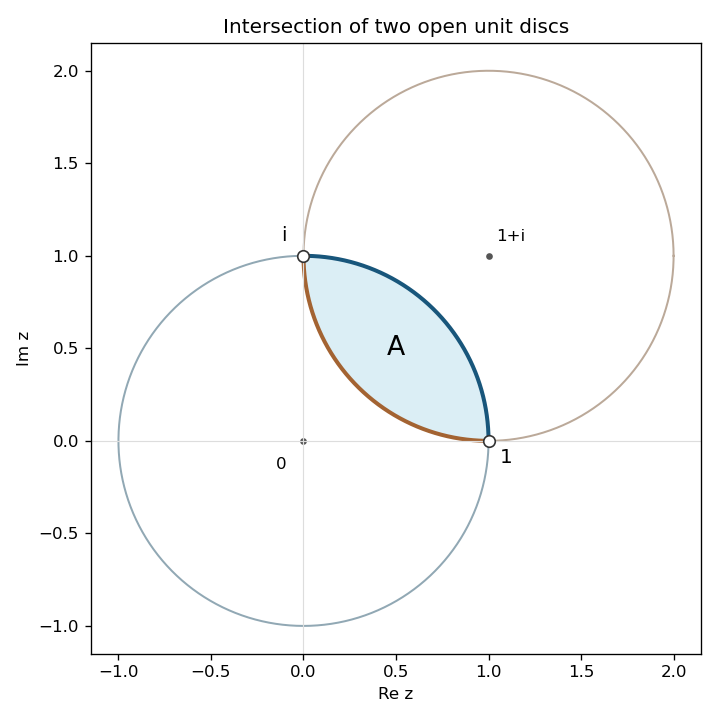


To construct a conformal map of a circular lens, apply the Möbius transformationIt sends the intersection points to zero and infinity, so both boundary circles become straight lines through zero. The boundary arc of the circle centred at zero maps to the ray of argument ; the other arc maps to the ray of argument . For example, their arc midpoints and give these signs. The interior point maps to one, selecting the sector , not the complementary sector. As a Möbius bijection, maps the whole lens onto that sector.
Squaring maps this sector bijectively onto the right half-plane: arguments double into , and the inverse is the unique square root with argument in . ThusThe derivative never vanishes inside the lens: and its derivative are nonzero there. Finally use the Cayley transform between the half-plane and disk . Since precisely when , it maps the right half-plane bijectively to the unit disc. The desired second map isThe denominator cannot vanish in the lens because has positive real part. The maps send the centre-line test point to one and zero respectively.
For a nonzero residue modulo an odd prime , the Legendre symbol equals if is a nonzero square modulo and otherwise. The extension to multiples of has value zero. Euler's criterion states
Apply Euler's criterion to . It givesFor , the same criterion gives . Both sides are integers in , which are distinct modulo an odd prime, so congruence implies equality. This proves multiplicativity of the Legendre symbol:
Since is nonzero modulo , it has a unique multiplicative inverse in the nonzero residues. The inverse cannot be because that would imply , excluded by the range. Thus as claimed. The congruence givesThe Legendre symbol of the nonzero square is one. Using multiplicativity of the Legendre symbol therefore gives
Inversion permutes the nonzero residues excluding . Hence the result of part (c) changes the requested sum intoThere are exactly nonzero squares: the map on nonzero residues identifies exactly the pairs , because implies in the finite field. Thus there are equally many nonzero squares and nonsquares, and the complete Legendre-symbol sum is zero. Removing the term leaves
The expectation value of an observable is the mean outcome of repeated measurements on identically prepared systems in the normalized state. For a self-adjoint it is real and equals . Assume the state belongs to the domains needed for the second moments and the commutator below, so all these quantities exist.
For real , positivity of the squared norm givesThe commutator expectation is purely imaginary, so this is a real quadratic in . If , its minimum is nonnegative exactly when its discriminant is nonpositive. If , nonnegativity for all real forces the linear coefficient to vanish, yielding the same conclusion. ThusReplace the observables by their centred versions , . Their commutator is unchanged, and their second moments are the variances . Taking square roots gives the Robertson uncertainty principleFor the quantum harmonic oscillator, gives . The uncentred inequality above consequently gives . The arithmetic-geometric mean inequality now yieldsThis is a bound for every normalized state of finite oscillator energy, not just an eigenstate. It is attained by the centred Gaussian ground state, for which and the uncertainty product equals .
Differentiability at means that there is a linear map such thatNecessarily when those partial derivatives exist. Under the stated assumptions, apply the one-variable mean value theorem separately to the two coordinate increments:for some intermediate , omitting a term if its increment is zero. Existence of the partial derivatives in a neighborhood supplies the differentiability along each segment required for that theorem. Their continuity at makes the difference from bounded by , where . Since , this is the required little-o remainder and proves Fréchet differentiability.
For the particular function, , so the defining difference quotients give . However for every . It is not continuous at the origin, and therefore not differentiable there. This illustrates why existence of partial derivatives alone is insufficient.
Let . A rotation matrix maps the unit sphere and its surface measure to themselves. Changing variables therefore gives , so is an isotropic second-rank tensor. Reflection symmetry also directly makes its off-diagonal entries zero, while interchange of coordinates makes its three diagonal entries equal. Its trace ishence . Oddness gives . Expanding the defining product for now givesThe action on a vector is . For , its eigenvalues and eigenspaces are thereforeThe latter has multiplicity two. If , the single eigenvalue has multiplicity three and every vector is an eigenvector apart from the excluded zero vector.
Assume the known variances are positive and write . The likelihood times the normal prior distribution is proportional toCollecting the quadratic and linear terms in completes the square with precision and mean . Thus normal-normal conjugacy givesFor quadratic loss, the posterior risk of reporting is , uniquely minimized at . For absolute-error loss, differentiating the posterior risk gives , so its minimizer is a posterior median. The normal posterior is symmetric about and has a strictly increasing distribution function, hence that median is uniquely . Therefore both optimal point estimates equal , the posterior mean.
For the cofinite topology , the empty set and are included. A nonempty union of cofinite sets is cofinite because its complement is contained in the finite complement of any one member. A finite intersection is cofinite because its complement is a finite union of finite sets; intersections involving the empty set are empty. This proves all topology axioms.
For the tail topology on the natural numbers , . Any nonempty collection of tails has a smallest starting index, so its union is that tail; a finite intersection of tails is the tail with largest starting index. Empty sets and empty-family conventions supply the remaining cases. Thus is also a topology.
We classify continuous maps between cofinite and tail topologies. Continuity is equivalent toIf has unbounded image, each is nonempty, hence cofinite. For every threshold , eventually , which is exactly . If the image is bounded, it is a nonempty finite subset of and has a maximum . Then is nonempty and cofinite, but always, so except at finitely many indices. These exhaust the two possibilities and prove necessity. Their sufficiency is checked separately below.
If , then for each the complement of contains only finitely many indices. Thus every nonempty open tail has a cofinite preimage, and the empty set has empty preimage. Hence is continuous from the cofinite space to the tail-topology space.
Suppose for all and eventually. If , then . If , the preimage contains all sufficiently large indices and is cofinite. Every open set therefore has open preimage, proving is continuous. Together with the introductory argument this proves the claimed if-and-only-if classification.
Eliminate the first entries of rows two, three and four using multipliers . All remaining subdiagonal entries are then already zero. The unit-lower-triangular LU decomposition isMultiplication verifies . Since , all pivots are nonzero. Forward substitution in givesBackward substitution in gives , , , and . ThusDirect substitution yields as a check.
Associate to the polynomial . The th component of is exactly . If , this polynomial of degree at most has distinct roots. Repeated use of the factor theorem would make divide any nonzero such polynomial, contradicting its degree. Hence is the zero polynomial and all . The converse is immediate, proving .
A square matrix has full column rank if and only if its kernel is zero, by rank-nullity theorem. Its row rank equals its column rank. Therefore this Vandermonde matrix has row rank , and its rows are a basis and span .
Take the unit circle counterclockwise and . The integrand is a Laurent polynomial with its only possible singularity at zero. Its expansion isThe term is the term , so the residue is . The residue theorem gives
Parametrize the same contour by , . Then and . Part a becomesCanceling the nonzero common factors gives
The positive-definite symmetric form is a real inner product. Choose a -orthonormal basis by the Gram-Schmidt process. The stated identity means that the matrix of satisfies . If , thenAn invertible has nonzero determinant, so is even.
To cover a possibly singular map, first show . If , then for every , giving one inclusion. Conversely orthogonality to the image gives for all , so nondegeneracy of gives . Positivity then implies .
The image is invariant under , and its restricted map is injective by that trivial intersection. In finite dimension it is consequently invertible. The restricted inner product is positive definite and the same skew-adjoint identity holds, so the first argument applied to this restriction makes even. Thusincluding rank zero. This is the even rank of a skew-adjoint linear map.
A Hermitian operator satisfies for all admissible states in its domain; in finite dimension this is . For an unbounded physical observable one specifies a self-adjoint realization, rather than only a formal differential expression.
Here and . For states with sufficient regularity and decay, integration by parts givesThe multiplication term cancels because is real. Thus the Quantum Hamiltonian is Hermitian on the stated admissible domain. Equivalent boundary conditions must remove this boundary term if the system is on a bounded interval.
The Schrödinger equation and its conjugate imply, for a time-independent observable and normalized state,This follows by differentiating both factors in and moving using Hermiticity. The canonical commutator givesConsequently the two Ehrenfest theorem identities areThey require the displayed expectations and domain operations to exist; real-valuedness of a potential alone is not a proof about every possible singular operator domain.
First is finite: by Cauchy-Schwarz, . It is nonnegative and absolutely homogeneous. If , every , so every column is zero and ; the converse is immediate. The triangle inequality for the Euclidean norm gives after taking suprema. Thus is a norm.
For any vector , rescaling gives . Applying this twice givesFurthermore , proving the requested strict entry bound when .
For a polynomial in matrix entries, expand each monomial at . The terms involving exactly one entry of give a linear map , with coefficients polynomial in the entries of . Every remaining term has at least two entries of and is for , because . This proves differentiability. Its derivative is continuous as an operator-valued function: each coefficient is continuous, and for every is bounded by one, so the operator-norm difference is bounded by the sum of the coefficient differences. Coordinate continuity follows from the same entry bound. Hence every such polynomial function is continuously differentiable.
In the Leibniz expansion of , the identity permutation supplies plus terms of degree at least two. Any nonidentity permutation moves at least two indices, so each of its terms has at least two entries. ConsequentlyIf is invertible, multiplicativity of the determinant and the preceding expansion giveThe adjugate identity gives . Thus for invertible .
For singular , take invertible , using the permitted density result. Both and the adjugate entries are continuous polynomial expressions, so taking limits for every fixed proves the derivative of the determinant formula on all matrices:Here the standard adjugate is the transpose of the cofactor array, as required by . In components this derivative is , also valid at singular matrices.
For an orthogonal change of Cartesian coordinates , an ordinary rank- tensor transforms byAn isotropic tensor is invariant under such rotations. Orthogonality gives , so transforming any of the three products of two Kronecker deltas leaves it unchanged. Their linear combination with arbitrary scalar coefficients is therefore isotropic.
For completeness, these three products exhaust the rank-four isotropic tensors in three dimensions. Half-turns about coordinate axes force a nonzero component to contain each coordinate label an even number of times. Axis interchanges then leave just the values , , and . Rotating the first two axes by gives , so . These component values are exactly those of the three-delta-product expression. Thus isotropy of the elastic medium gives this form for its elasticity tensor.
Contracting with the symmetric strain givesThese are the Lamé parameters. Taking the trace determines the scalar part of the strain:Since , the stored strain energy density isA nonzero traceless test strain proves necessity of , and a pure scalar strain proves necessity of . Conversely these two conditions make both terms nonnegative for every strain. Thus nonnegative isotropic elastic strain energy is equivalent to
Model the two samples as independent multinomial counts with fixed row totals and three category probabilities. The null hypothesis is for every category . Up to combinatorial factors the likelihood is . Without the null restriction its maximizers are ; under the null, maximizing subject to givesThe observed column totals are , giving fitted expected counts in each row.
To derive the null distribution, put . Under the null its mean is zero and covariance is . The multivariate central limit theorem gives, asymptotically, the standardized contrast a centered normal distribution with covarianceThis is the orthogonal projection onto a two-dimensional plane. In an orthonormal basis of that plane, the two nonzero coordinates are independent standard normal variables, so tends to . The pooled estimates are consistent; substituting them for leaves this limit unchanged by Slutsky's theorem. Since and , the resulting statistic is precisely the Pearson chi-squared test of homogeneity statisticThis supplies the two degrees of freedom rather than treating all six cells as independent. Every fitted expected count is large, supporting the approximation.
For these data,It exceeds the two-degree-of-freedom 95th percentile , but not the 99th percentile . Hence reject equal score distributions at the 5% level, but not at the 1% level. The asymptotic p-value is .
Define by for and . It is continuous away from zero, and , so it is continuous at zero too. Its image is exactly , using . The interval is compact, so its continuous image is compact.
For any two image points , the explicit pathis continuous and joins them. Thus the reciprocal spiral with its endpoint is also path-connected. Infinite winding causes no discontinuity at the endpoint because its radius tends to zero.
The set is path-connected as the continuous image of , hence connected. Its closure is together with the unit circle. Indeed as , and any convergent sequence of spiral points either has bounded parameters, giving a point of , or has parameters tending to infinity along a subsequence, giving radius one. The closure of a connected set is connected: a separation of its closure would induce a separation of the dense original set, with neither open part missing that set. The closed disk is connected and meets this closure in the unit circle; their union is therefore connected.
To show it is not path-connected, suppose a path starts in and ends in the disk. Let be its first contact with the disk. The disk is closed, so this first contact exists, and . Before it, the path belongs to and has a continuous uniquely determined parameterContinuity at contact forces , and hence as . The intermediate value theorem supplies times approaching at which is an integer, and other times at which it is an integer plus . These times must approach contact because is bounded on every compact interval strictly before it. Along the first sequence ; along the second it tends to . This contradicts continuity at . Thus no path joins the spiral to the disk, proving failure of path-connectedness for the spiral accumulating on a circle.
Exactness on the polynomial basis requiresSolving givesThus the approximation is the unit-spacing centered second difference, .
Articles were limited to the first 100 out of 269 total.
Articles by others on the same topic
There are currently no matching articles.