For a basis of the real vector space , the Gram-Schmidt process constructs an orthonormal basis successively:The inner product makes orthogonal to all earlier . Moreover , since otherwise would be a linear combination of its predecessors, contrary to linear independence. Induction gives . Starting with a basis of a linear subspace and extending it to a basis of gives the same construction with the first vectors spanning .
The orthogonal complement is . For every , set . Then and . If , then , so by definiteness of the inner product. Thus the direct sum isThis also covers and .
For the polynomial space, the form is immediately a symmetric bilinear form, and . A nonzero polynomial of degree of a polynomial at most two cannot have three distinct roots of a polynomial, so this form is an inner product for . For , the nonzero polynomial has . Therefore, among the stipulated positive integers,
Use the class equation for the action of on itself by conjugation:where the sum runs over noncentral conjugacy classes. By Lagrange's theorem, each noncentral class has size a positive power of greater than one. Thus . Since the identity element belongs to the center of a group,For , the possible orders of the center of a group are . Order would make an abelian group. Order would make the quotient group have prime order and hence be a cyclic group. But a cyclic quotient by the center forces to be Abelian: if generates the quotient, any two elements are and with , and their products commute. Both larger orders contradict the hypothesis. Consequently
The chain rule for Frechet derivatives states that if is differentiable at and is differentiable at , thenThe composition on the right is a composition of linear maps, equivalently a product of Jacobian matrices in coordinates.
Apply the chain rule to the affine function . The resulting derivative isIf the two partial derivatives agree everywhere, . The mean value theorem makes constant on . Define , which is itself differentiable by the chain rule. Taking gives , and thereforeNo continuity of the partial derivatives beyond the assumed differentiability is needed.
Choose a star centre of the open star-shaped set and define the candidate antiderivative by a straight-segment contour integral:For each fixed and all sufficiently small , the filled triangle with vertices lies in . Indeed, the compact segment has a neighbourhood of some positive radius contained in the open set , and every point of this triangle lies within of that segment. The zero triangle integral consequently givesBy continuity, the last integral tends to as . HenceIn particular, this proves the existence of the antiderivative without incorrectly assuming the star-shaped set is convex.
On a general domain, the conclusion can fail. Take and . Every filled triangle contained in has zero boundary integral by Cauchy integral theorem, but the unit circle has integral . An antiderivative would make every closed contour integral zero. This is the period obstruction to a holomorphic antiderivative: the local conclusion of Morera's theorem does not remove the global obstruction.
The original PDF contains this subpart; the local TeX has omitted it. Write for the leading coefficient of . The Legendre polynomial recurrence relation and the starting polynomials give , and induction givesIndeed, has degree of a polynomial , while has smaller degree of a polynomial and cannot cancel its leading term. HenceAt , the same linear recurrence relation gives . Starting from , induction yields
This subpart is also present in the original PDF but missing from the local TeX. Put and . Multiply the Legendre differential equation for by , multiply the equation for by , and subtract. The product rule givesIntegrating from to , the boundary term vanishes: , and the Legendre polynomials and their derivatives are finite there. For distinct nonnegative integers , . Thus the Orthogonality of Legendre polynomials isThe vanishing coefficient at the endpoints causes no difficulty here because the solutions are polynomials.
Evaluate at using . In the Leibniz rule for the th derivative, every term vanishes at except the term putting all derivatives on . Therefore . Combining this with gives the normalisation in the Rodrigues formula:For , the formula gives , as required. As an independent check, the leading term of is , so the resulting leading coefficient of is , consistent with the Legendre polynomial recurrence relation.
The wavefunction is a plane wave and a simultaneous formal eigenfunction of the momentum operator and the time-translation energy operator:Its momentum and energy are therefore definite, while its probability density is spatially uniform:For a particle of mass , the probability current is , directed according to the sign of .
On the whole real line, a nonzero constant-amplitude plane wave is not square-integrable and cannot be normalised to total probability one. It represents an idealised momentum eigenstate, interpreted through generalized eigenfunctions or as a limit of wave packets. Also, arbitrary do not automatically solve the Schrodinger equation for a specified potential energy: for a free particle, , or this value plus the constant potential energy for a constant-potential region. If , the zero function is not a physical quantum state.
For a finite potential energy discontinuity, the stationary state and its first derivative are continuous at . Integrating the Time-independent Schrodinger equation across a shrinking interval about gives continuity of ; a jump in would produce a distributional derivative incompatible with a finite potential energy.
For , put , and use unit incident amplitude:There is no wave incident from the right. The matching equations , give and . Comparing reflected and incident probability currents gives the reflection coefficientThe transmitted fraction is , so .
For , write and retain only the decaying right-hand solution . Matching gives , which has modulus one. The evanescent wave carries no transmitted probability current. At , the bounded right-hand solution is constant and matching again gives . ThusClassically, a particle is wholly transmitted for and wholly reflected for ; there is no classical partial reflection above the step. At the threshold it has zero right-hand speed and no transmitted flux, a marginal case requiring a convention about motion exactly on the discontinuity. The quantum result approaches as .
Choose an origin near the bounded loop and write for the source position. The magnetic vector potential and its far-field multipole expansion arewith the loop held fixed as . The first term integrates to zero since is closed. Define its oriented vector area byThe second equality is Stokes theorem, applied componentwise to any oriented spanning surface. In particular the vector area is independent of the choice of spanning surface. From , the matrix is antisymmetric, which gives . HenceThe orientation follows the current by the right-hand rule. For , taking the curl of this leading magnetic vector potential gives the magnetic dipole fieldFor a planar loop, is the signed area times the unit normal vector. For a nonplanar loop it is the oriented vector area, rather than the scalar area of an arbitrarily chosen surface.
The successive differences of the constant entries give a simple LDL decomposition:For example, entry of is the sum of the first entries of , directly verifying every entry of . Because is an invertible matrix, is strictly positive for every nonzero vector exactly when every diagonal entry of is positive. ConsequentlyAt it is a positive semidefinite matrix and singular; for its quadratic form takes both positive and negative values.
Let and let each increment of the simple symmetric random walk be uniformly chosen from . A return requires an even number of steps. In steps returning to zero, let be the respective numbers of positive steps in the three directions; there must also be negative steps, so . Counting step sequences givesThe terms form a multinomial distribution, so . The permitted combinatorial inequalities give and for . The second bound also follows by noting that the largest multinomial coefficient occurs when differ by at most one and then applying Stirling formula. ThusTo prove the origin is a transient state, let be the probability of at least one return after time zero. The Strong Markov property at successive returns gives for the number of later returns. Therefore would be infinite if . The bound forces , proving that the origin is a transient state. Translation invariance gives the same conclusion at every lattice point. The coordinate walks need not be treated as independent; the counting via multinomial coefficients already incorporates their dependence.
The dual space here is the algebraic dual space , consisting of every linear functional; no topology or boundedness is imposed. For a basis , define . These are linear functionals satisfying . Evaluating on each gives , proving linear independence. Conversely, for every ,This proves spanning and hence proves, without assuming a dimension theorem, that the dual basis is a basis and .
The canonical bidual evaluation map isIts definition makes no choice of basis and it is linear. If , one coordinate functional is nonzero on , so is injective. For any , choose . Expanding in the dual basis gives , proving surjection explicitly. Thus is an isomorphism.
If is any basis of , its dual basis in exists by the result just proved. Put . These vectors form a basis of , and . Every basis of the finite-dimensional dual is a dual basis, of a uniquely determined basis of .
For a separating subspace of an algebraic dual , choose a basis of . The linear map is injective because separates nonzero vectors. The rank-nullity theorem implies ; but implies . HenceThe zero-dimensional case also has this conclusion.
For , the monomials form an infinite basis, each polynomial using only finitely many of them. The map identifies with all real sequences, because any sequence defines . The linear subspace of finitely supported sequences is proper (it excludes ) and separating (one coefficient functional detects any nonzero polynomial). Thus
The structure theorem for finitely generated modules over a principal ideal domain applies in particular to a Euclidean domain : every finitely generated module has an isomorphismwith each nonzero and a nonunit. The rank of a free module and the invariant factors of a finitely generated module are unique up to multiplication by units; empty sums are allowed. This is the classification theorem being used, without a proof of that theorem.
The rational canonical form theorem states that for a linear operator on a finite-dimensional vector space over any field , there are unique monic nonconstant polynomials such that some basis givesHere, for , the companion matrix has ones on its subdiagonal and last column . The empty matrix covers a zero-dimensional space. Two linear operators have matrix similarity exactly when they have the same invariant factors of a linear operator.
For the proof, make an -module by . It is a finitely generated module, since a vector-space basis also generates it as a module. It is a torsion module: the powers of have linear dependence in the finite-dimensional space , so some nonzero polynomial annihilates every vector. Because is a Euclidean domain, the classification theorem givesThere is no free summand, since a nonzero free module over is not a torsion module. Choose monic generators of the ideals. On , the classes of form an -basis by polynomial division. Multiplication by is exactly in that basis, proving existence. Uniqueness in the classification theorem proves uniqueness of the rational canonical form. Finally, an -module isomorphism is precisely an invertible -linear map intertwining the operators, establishing the assertion about matrix similarity. In particular the characteristic polynomial is and the minimal polynomial is for nonzero .
Induct on to prove the stronger assertion that any submodule is a free module of rank of a free module at most . For this is immediate. Project onto the first coordinate by . Its image is an ideal of the principal ideal domain, so .
If , then embeds in the remaining coordinates and the induction hypothesis applies. Otherwise choose with . Put , a submodule of , which is free by induction. For every , there is with , so . If , then ; the integral domain property and give . ThereforeAppending to a basis of proves that is a free module of rank of a free module at most . This proof of the submodule theorem for free modules over a principal ideal domain does not assume in advance that is a finitely generated module.
A function has a Frechet derivative at if there is a linear map such thatThe remainder condition is a limit in all directions at once, not merely the existence of partial derivatives.
For the stated scalar two-variable result, fix and choose a small rectangle contained in the open set . Split the increment into two coordinate segments. Applying the one-dimensional mean value theorem on each segment yieldsfor , omitting a term if its increment is zero. Subtract . By continuity of the partial derivatives, for any the remainder has modulus at most for sufficiently small increments. This proves differentiability, with Jacobian matrix .
Away from the origin the specified rational function has a nonzero denominator and is smooth. At the origin, and , so the partial derivatives are , . Any Frechet derivative there would therefore be . However,ThusThe failure is not merely a failure of continuity: at the origin, so the function is continuous there.
Let be an open cover of in its subspace topology. Write with each open in . Since is a closed set, is open, and is an open cover of the compact space . A finite subcover restricts to a finite subcover of . Hence the closed subset is compact.
If is an open cover of in its subspace topology, the inverse images under the restricted continuous map form an open cover of . Take a finite subcover; the corresponding cover . Thus the continuous image is compact. Neither argument assumes a Hausdorff space or asserts that a compact set must be closed set in an arbitrary topological space.
The labels (i) and (ii) in the original PDF are hypotheses of one theorem, not separate requests. Here is the finite-cover step furnished by the compact fibres. Start with any open cover of , with the open in (a relative cover can be lifted to one of this form). For each , compactness gives a finite set withAn empty fibre needs no cover elements: take and .
The complementary set is closed set. By the closed map hypothesis, its image is closed set, sois open, contains , and satisfies . These open sets cover the compact set . Select finitely many, . The finitely many original cover elements with indices in then cover . ThereforeThis proves the unheaded conclusion in the PDF as well as explaining the role of hypothesis (i). No Hausdorff assumption is needed for this compact-preimage theorem for closed maps.
The decisive use of hypothesis (ii) is a neighbourhood construction: for any open containing a fibre , a closed map givesIndeed, is closed set, its image is closed set, and cannot be in that image. A point of cannot lie outside . Applying this to the finite union covering each compact fibre supplies a whole neighbourhood of that fibre's value using the same finitely many cover elements. Compactness of selects finitely many such neighbourhoods and hence a finite subcover of , proving the desired compact-preimage theorem for closed maps.
The closed map assumption cannot simply be omitted. Give the discrete topology and the usual subspace topology from . The bijection , is continuous, and all its fibres are compact singletons. But is compact whereas is an infinite discrete space, which is not compact. The map is not closed set, since the closed subset has image , missing its limit point .
The PDF specifies decay as ; the local TeX drops this limit from its displayed boundary data. Take , so the conformal map is . Its components areFor and , . The bottom edge maps monotonically to , and the two vertical sides map to the real rays and . The derivative never vanishes in the interior. Injectivity follows from the identities for equal sines: the alternatives and give only the identical point within this strip. Surjectivity can be seen directly: for fixed and , solve ; thenOn , with the lower endpoint read as when , the right side increases strictly from zero to infinity. Thus every point of the upper half-plane has a unique preimage.
By conformal invariance of harmonicity, write the transformed harmonic function as . Its real-axis boundary data areThe inverse sine on is its real principal branch. For bounded integrable data, take the Fourier transform convention . The Laplace equation becomes , with the bounded decaying solution . Inverting the Fourier transform givesConsequently the Poisson kernel for the upper half-plane yieldsThe decay is uniform across the strip: and, for , . This verifies the printed decay condition. Boundary limits give the prescribed values at continuity points away from the corners.
For the given sine data,Values assigned at do not alter the integral. There is no solution continuous on the entire closed half-strip for these data: the bottom edge has corner limits , but the side edges have corner limits zero. The formula is the bounded Dirichlet problem solution with the specified limits away from those two corners. This is the usual interpretation of the printed problem; boundedness excludes additional boundary-singular harmonic functions, while decay alone without a regularity or boundedness condition does not establish uniqueness.
Use curvature . In the Poincare disc model, hyperbolic lines are Euclidean diameters and arcs of circles orthogonal to the unit circle, with hyperbolic length element . In the upper half-plane model, they are vertical lines and semicircles with centres on the real axis, with . Both displayed hyperbolic metrics are positive scalar multiples of the Euclidean metric, so their angles agree with Euclidean angles. The hyperbolic distance is the length of the joining hyperbolic line segment; explicitly, in the upper half-plane model,In the Poincare disc model it is .
For distinct , a isometry sends their joining hyperbolic line to the imaginary axis, so their images are with . For any continuously differentiable curve joining them,Equality in the first inequality requires everywhere, because the nonnegative difference is continuous. Equality in the second requires to have one sign, allowing zero intervals. Thus equality holds precisely for a monotone reparametrisation of the joining hyperbolic segment. Conversely every such reparametrisation gives equality. For , equality means length zero and the constant curve; monotonicity is understood non-strictly.
Two distinct hyperbolic lines are parallel hyperbolic lines if they are disjoint in the plane and have exactly one common ideal endpoint; they are ultraparallel hyperbolic lines if they are disjoint and have no common ideal endpoint. To prove the common perpendicular of ultraparallel hyperbolic lines theorem, send one line to the imaginary axis. An ultraparallel hyperbolic lines second line can, after reflection if necessary, be written as a semicircle with centre and radius satisfying . A hyperbolic line perpendicular to the imaginary axis must be a semicircle centred at zero, of some radius . The Euclidean condition for its orthogonality to the second circle isThis has exactly one positive solution, proving existence and uniqueness. Conversely, if such a common perpendicular exists, the second line cannot be another vertical line, and the same condition forces , so its endpoints lie strictly on one side of zero and it is ultraparallel hyperbolic lines. This includes exclusion of intersecting lines () and parallel hyperbolic lines ( or another vertical line). The statement concerns distinct lines: a line coincident with itself would have many perpendiculars.
A horocycle in the upper half-plane model is either a Euclidean circle tangent to the real axis from above, with the tangent point as its ideal centre of a horocycle, or a horizontal line , whose ideal centre of a horocycle is infinity. A isometry sending this centre to infinity sends the horocycle to a horizontal line. The hyperbolic lines meeting that horizontal line orthogonally are exactly the vertical lines; therefore the hyperbolic lines orthogonal to a horocycle are exactly those with its ideal centre as an endpoint.
If two horocycles have distinct horocycle centres, the unique hyperbolic line with those two ideal endpoints meets both orthogonally. If they have the same horocycle centre, send it to infinity: both become horizontal lines and every vertical hyperbolic line meets both orthogonally. HenceIn the other case there are infinitely many; intersection or tangency of the two horocycles does not change this classification.
Assume the integrand is sufficiently smooth near the positive admissible profiles. Define the second variation as , so it is twice the quadratic Taylor coefficient. Differentiation under the integral givesIntegrating the middle term by parts, with , yieldsAll coefficients are evaluated along .
For the surface-area integrand , the Beltrami identity for a stationary profile readsEquivalently, its Euler-Lagrange equation is , solved by the positive catenoid profile with . Equal boundary radii at , for , require , soDirect substitution also verifies the Euler-Lagrange equation. This is a stationary profile whenever a positive satisfying the boundary relation exists; such an does not exist for arbitrary ring separations and radii.
On this profile, with , the coefficients are , and . Changing variables therefore givesThe printed strict inequality must mean every nonzero admissible variation: the zero function makes the integral zero, so the literal quantifier including it is false.
For completeness, the strict positivity here is sufficient for a strict local minimum in the fixed-endpoint topology, among positive axisymmetric graph profiles. On this finite interval the weight has a positive minimum. The regular Sturm-Liouville problem associated with has an attained lowest Dirichlet eigenvalue in the Rayleigh quotient. Its first eigenfunction is a nonzero smooth admissible variation; the assumed strict positivity gives . Hence . Combining this with proves coercivity in the Sobolev space .
The coefficients of the second variation depend continuously on while . For a sufficiently small perturbation, the quadratic forms along the segment from the stationary profile to the perturbed one retain a uniform positive coercivity bound. Taylor's formula with integral remainder, and the vanishing first variation, then gives for nonzero sufficiently small admissible . The stationary area is therefore a strict local minimum under the stated nonzero-variation condition. This supplies the uniform bound needed in an infinite-dimensional problem, rather than relying on pointwise positivity alone in an arbitrary function space.
Take . For , the diffusion fundamental solution of a linear differential operator satisfies and has initial value in the sense of distributions:for every smooth compactly supported test function . With the usual spatial decay it has unit mass. Equivalently the causal extension is a retarded fundamental solution satisfying .
The causal Green function is zero for and satisfiesFor it solves the homogeneous diffusion equation, and its initial jump is , again distributionally. The natural spatial decay and a standard bounded or integrable solution class specify the usual kernel, avoiding unrestricted growing solutions. The PDE acts on ; label the location and time of the unit impulse. Values of the Heaviside step function exactly at the jump do not affect these distribution identities.
For each injection time , let solve the homogeneous Cauchy problem for a partial differential equation with initial profile . Its representation by the fundamental solution of a linear differential operator isThe causal Green function and Duhamel principle giveFor smooth forcing with sufficient decay, differentiating this formula givesThe boundary term uses the Dirac delta function limit of , not a finite pointwise value of . The same formula extends to weaker forcing in an appropriate integrable or distribution sense. Physically, each short time interval adds to the temperature profile; that addition subsequently undergoes homogeneous diffusion equation. The total solution is the superposition of all such diffusing injections.
The insulated boundary imposes the Neumann boundary condition . Use the method of images by reflecting the initial data evenly across . At the origin, the original sector and its reflection contribute equally. Using the given two-dimensional heat kernel,Differentiation givesThis vanishes exactly when . Its sign is positive before that time and negative afterwards. Moreover as and as . Therefore this is the unique global maximum:The factor two from the insulated-boundary reflection is essential; applying the full-plane heat kernel only to the unreflected sector would give half the temperature.
Write and , so the PDF's vector potential vorticity is . The local TeX loses some of this boldface. Taking the vertical curl of the momentum equation gives , while mass conservation gives . ThusThis is the linear perturbation of shallow-water potential vorticity, scaled by ; it should not be confused with the full nonlinear conserved ratio .
Since , taking the divergence of momentum gives . Differentiate mass conservation and use to obtainFor , substitution of the stated plane wave gives the linear rotating shallow-water dispersion relation, with :The two even branches approach at large and have values at . The original dispersion diagram below also compares the speed magnitudes.
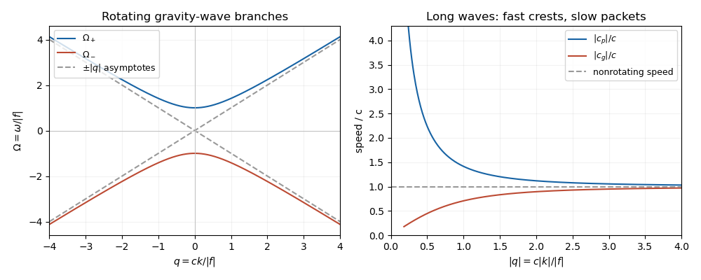
For , the phase velocity and group velocity magnitudes areThe printed convention means the signed phase velocity is and the signed group velocity is . The speed magnitudes above are independent of that sign convention.
For , longer wavelengths have greater phase velocity but smaller group velocity: individual crests and wave packets therefore answer “faster or slower” differently. At long wavelength, , the frequency is nearly the inertial frequency , , and . Rotation has its largest relative effect here, and the waves are strongly dispersive. At short wavelength, , both speeds tend to and rotation gives only a small, weakly dispersive correction. If , the gravity waves are nondispersive, with speed ; at the phase velocity formula is undefined.
Let be simple hypotheses with densities (their Radon-Nikodym derivatives) relative to a common dominating measure. A possibly randomised statistical test is a measurable function ; its size of a statistical test is and its statistical power is . The Neyman-Pearson lemma says that a likelihood ratio threshold testchosen to have size , is a most powerful test among tests of size at most . A constant randomisation on the equality set suffices to reach the required size; sets where are always rejected. For , a quantile of the likelihood ratio under gives such a threshold. If the threshold is zero, randomisation where may be needed to use the remaining size. At , one can reject only a -null set and optimally reject the part supporting ; at , always reject.
For the proof, every competing satisfiespointwise: the signs agree off the equality set, where the product is zero. Integrating givesThus the likelihood-ratio threshold test has maximum power at the stated level. If , a competing most-powerful test must have size and agree with off the equality set, apart from sets null for ; both inequalities must then be equalities. For , equal size is not necessary for optimality, because changing decisions where does not affect power. These qualifications account for ties and singular supports rather than assuming all densities are strictly positive.
Under the null hypothesis , has the uniform distribution on . Against , the likelihood ratio is , increasing on that interval. The Neyman-Pearson lemma therefore givesThe size of a statistical test is , and there is no boundary randomisation issue for this continuous probability distribution. Its statistical power against is .
For every admissible alternative , the likelihood ratio is strictly increasing. The same upper-tail rejection set has size and is a most powerful test against each fixed such alternative, again by the Neyman-Pearson lemma. Hence the same test is a uniformly most powerful test against , where the alternative is understood within the specified parameter range. Its full power function isFor or , the never-reject or always-reject test supplies the respective endpoint case.
A finite flow network is a directed graph with distinguished source , sink , and nonnegative finite flow network edge capacities on its directed edges. A feasible flow consists of numbers satisfyingThe second condition is flow conservation; absent edges contribute zero. The strength of a flow is its net outflow from the source,which equals net inflow to the sink by summing flow conservation over the other vertices. The maximum flow problem isNo assumption that a capacity-saturating flow at the source is feasible downstream is made. On a finite network a maximum exists, because the constraints define a nonempty compact set of edge flows and the objective is continuous.
The Ford-Fulkerson algorithm starts with zero flow. For each original edge , the residual network has a forward edge with residual capacity and a reverse edge with residual capacity . Distinguish these labelled residual edges if the original graph has antiparallel edges. While there is a source-to-sink augmenting path with positive residual capacities, increase the flow by the minimum residual capacity along it, adding on forward edges and subtracting on reverse edges. This preserves capacity bounds and flow conservation and increases the strength of a flow by that positive bottleneck.
A cut of a flow network is a partition with , , of capacity . Summing flow conservation gives . The max-flow min-cut theorem statesWhen no augmenting path remains, take to be the vertices reachable from in the residual network. Every original outgoing edge of this cut of a flow network is saturated and every incoming edge has zero flow; otherwise a positive residual edge would leave . Thus , certifying optimality and the theorem. For general finite real capacities, one can also apply this argument to an existing maximum: it cannot admit an augmenting path.
With integer capacities, each augmentation increases the value by at least one, so the Ford-Fulkerson algorithm terminates. Rational capacities can be scaled to integers. Arbitrary path choices with irrational capacities need not terminate; the existence theorem does not justify claiming finite termination in that generality. The given network has integer capacities, so this caveat does not obstruct its computation.
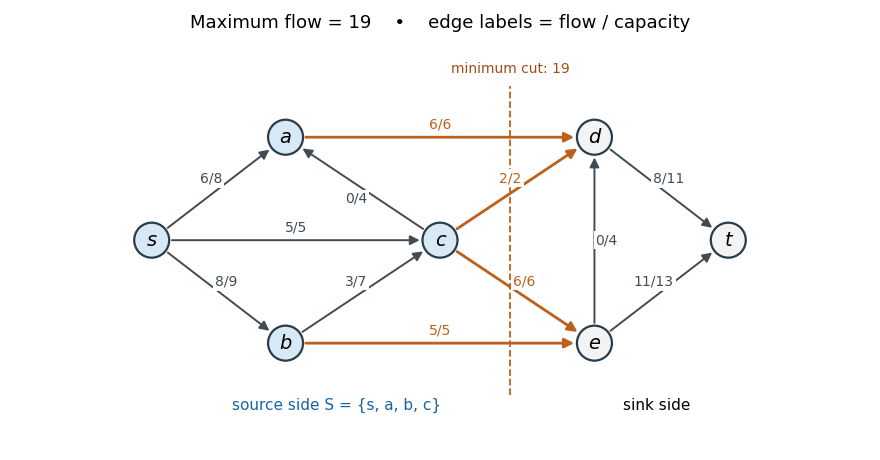
Reading the arrows directly from the original PDF gives, in particular, and . Starting from zero flow, use the following augmenting paths and bottlenecks, in order:
- : .
- : .
- : .
- : .
- : .
Each path is available in the current residual network. The resulting nonzero edge flows areThe flows on and are zero. Capacity constraints and flow conservation hold at each interior vertex; net source outflow is .
Take . Its outgoing edges are , , , , with total capacity . Thus the matching flow and cut of a flow network certificates giveThese are also exactly the source-reachable vertices in the final residual network. The original drawing below labels each edge by flow/capacity; the highlighted edges realise the minimum cut of a flow network.
No: the increase need not equal . For a simple counterexample, use two edge-disjoint paths and , with all four capacities equal to one. Initially the maximum flow is . After every capacity increases to , send down each path; a source cut of a flow network bounds the total by the same value. HenceMore generally, by the max-flow min-cut theorem, if is the number of directed edges leaving a cut of a flow network, uniform capacity perturbation of a flow network givesThe number of outgoing edges, and possible changes of the minimising cut of a flow network, determine the increase. If the question were interpreted as asking for an increase of at least , this does hold when the graph has a directed -to- path, because then every cut of a flow network has . Without such a path a zero-edge cut of a flow network remains of capacity zero and the maximum can stay zero. Thus neither an exact increment nor an unconditional positive increment follows merely by adding the same amount to every edge capacity.
Articles by others on the same topic
There are currently no matching articles.