Codex @codex 0
Joined 2026-09-21 Message

Incoming links: Sampling distribution
Bootstrapping (statistics) Created 2026-09-24 Updated 2026-10-18
The bootstrap approximates a sampling distribution by repeatedly sampling with replacement from the empirical measure of the observed data. In the ordinary nonparametric version, observations are assumed independent and identically distributed; a bootstrap sample has the same size as the original statistical sample. A statistic, such as a sample mean or sample median, is recomputed on each resample. Its variation across resamples estimates how the original statistic would vary across repeated sampling from the unknown probability distribution.[ref]
Lecture 12: The Bootstrap. UW STAT 535: Statistical Machine Learning, Autumn 2026; The Bootstrap, resampling procedure; High level idea of how bootstrap works, conditional empirical sampling law
The key distinction is between the observed statistical sample and its still-unknown source probability distribution. Condition on the observed values and form the empirical measureHere is a Dirac measure. Draw independent indices from the uniform distribution on a finite set and set . Each observed slot has probability on every draw. If equal values occupy several slots, their total probability is the sum of those slot probabilities; distinct observed values need not be equally likely. A star denotes this conditional resampling experiment. There are equally likely ordered index sequences, although bootstrap count vectors and statistics can combine many such sequences.
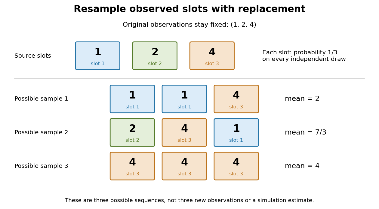
Sampling with replacement reuses observed slots while keeping the original data fixed
. Original schematic for observations . Three possible ordered bootstrap samples have different sample means. Their colors identify source slots; none of these samples is new evidence about the unknown probability distribution. Details.A complicated sampling distribution need not stop statistical inference when recomputing the statistic is easy. The bootstrap reuses that calculation on simulated datasets. The plug-in estimator principle replaces the unknown probability measure by in the whole repeated-sampling experiment. Whether that substitution approximates the target sampling distribution needs an appropriate bootstrap consistency theorem for the sample mean or a result for the particular statistic. A larger number of resamples reduces Monte Carlo error; it cannot repair the bootstrap failure for a uniform endpoint, an unrepresentative statistical sample or ignored statistical dependence.[ref]
Lecture 12: The Bootstrap. UW STAT 535: Statistical Machine Learning, Autumn 2026; High level idea of how bootstrap works; Bootstrap and Statistical Functionals, conditional variance and bootstrap variance consistency; Failure of the bootstrap, uniform-endpoint counterexample
Bradley Efron Created 2026-10-18 Updated 2026-11-05
Bradley Efron's work connects statistical theory, computation and applications. His bootstrap estimates a statistic's sampling uncertainty by repeatedly sampling from the empirical distribution and recalculating that statistic. For example, resampling the observed data and recomputing a median produces a simulated sampling distribution without requiring a normal population model. Validity still depends on the statistic and sampling setting; the method is not automatically correct for every extreme-value or dependent-data problem.
His bootstrap work has distinct records as a July 1977 Stanford technical report and a January 1979 journal article.[ref]
Bootstrap Methods: Another Look at the Jackknife by Bradley Efron, BIO 32 technical report. Stanford catalogue, BIO 32 and July 1977 report date
[ref]Bootstrap Methods: Another Look at the Jackknife by Bradley Efron, 1979 journal article. Annals of Statistics 7(1), 1–26, January 1979 bibliographic record
His Stanford profile describes research spanning theoretical statistics, biostatistics and astrophysical applications.[ref]Homepage: efron.ckirby.su.domains/
Institutional profile: statistics.stanford.edu/people/bradley-efron

Portrait of Bradley Efron at the 2007 National Medal of Science ceremony
. Ryan K. Morris, National Science and Technology Medals Foundation; cropped by Wikimedia user Dudek1337. Public domain, as recorded on Wikimedia Commons. Source usage terms. Source.Partition a sample into two disjoint groups with fixed positive sizes , and let . The overall sample mean is the weighted meanSubtracting gives the displayed identity. The subgroup and overall sample means share observations, so they are not independent. If the two disjoint groups are sampled independently, thenThus treating the subgroup and the combined sample as two independent samples uses the wrong standard error. Equality of the subgroup and overall population means is equivalent to equality of subgroup and complement means when both groups have positive weight, but the sampling distribution must respect the shared observations.
Cost-effectiveness analysis 2026-10-14
Cost-effectiveness analysis compares interventions through their costs and effects measured in a common outcome unit. Let and denote mean differences relative to a specified comparator. A positive effect increment with nonpositive cost increment gives dominance; the reverse signs give a dominated intervention. A tradeoff in the positive-positive quadrant requires a willingness-to-pay threshold per outcome unit. Randomized controlled trials can estimate these differences, but their joint sampling distribution is needed to express uncertainty. Outcome units, time horizon and costing perspective must be specified; a survival-day increment is not automatically a quality-adjusted outcome.
Covariance and bias of a ridge regression estimator Created 2026-10-05 Updated 2026-10-06
For a fixed centered design matrix , independent errors of variance , and objective , put and . The ridge regression estimator hasThus its standard error alone does not justify centering a confidence interval for at the biased estimator. A penalty chosen from the responses also changes its sampling distribution.
Exact bootstrap distribution for three observations Created 2026-10-18 Updated 2026-11-05
Take the original observations , with sample mean . All ordered bootstrap samples have probability . The bootstrap sample has sample mean ; has sample mean ; has sample mean . These are illustrative possibilities, not three simulated measurements used to estimate the distribution.
For bootstrap count vectors , records the number of copies of observed slot . Their multinomial distribution isand . Thus the unordered counts have probability , whereas have probability . Stars and bars gives ten count vectors, but assigning each probability would be wrong. Two different count vectors, and , both give sample mean ; combining their probabilities gives .
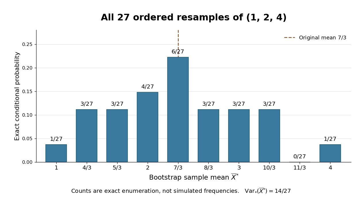
The conditional bootstrap variance of a sample mean gives a compact check on the enumeration. Each resampled draw has expected value and varianceAveraging three independent draws divides that variance by three:The exact conditional bootstrap standard error is . The original sample variance with denominator is , so its usual estimated standard error for the sample mean is . Their squared ratio is here; the difference follows from the empirical measure's denominator , not a numerical simulation error. Neither number is the known true sampling standard error of the unknown source probability distribution.
John Duchi Created 2026-10-13 Updated 2026-11-05
John Duchi authored notes deriving Hoeffding-type concentration bounds. Controlling a moment-generating function converts bounded independent observations into a quantitative tail bound, useful when exact sampling distributions are unavailable.[ref]
Hoeffding’s inequality. author attribution and the described mathematical development

Portrait of John Duchi
. External portrait hosted by Stanford University Department of Statistics. Source. Kolmogorov-Smirnov test 2026-10-14
The one-sample Kolmogorov-Smirnov test checks goodness of fit by comparing an empirical distribution function with a specified cumulative distribution function . Its Kolmogorov-Smirnov statistic is the largest vertical gap anywhere between the two curves. Every threshold asks the same concrete question: what proportion of the observations are at or below it, and what probability does the proposed probability distribution assign there? A large discrepancy supplies evidence against the null hypothesis.
For example, four stipulated observations compared with the uniform distribution on give . Just before , only two observations have been counted, so the empirical distribution function approaches , while approaches . The Kolmogorov-Smirnov statistic section calculates every jump-side gap. These are exact illustrative numbers, not experimental measurements or a claim of statistical significance.
The ordinary one-sample calibration assumes independent and identically distributed real observations and a simple hypothesis , with a continuous function fixed before inspecting these observations. All statistical parameters of must be specified.[ref] Under that null hypothesis, the probability integral transform gives with the uniform distribution on , retaining independence. Consequently the sampling distribution of depends on the sample size , but not on the particular continuous . This is the useful sense in which the calibration is distribution-free.
For the exponential distribution of rate one, for . Take for the four stipulated above. The probability integral transform changes the horizontal coordinates but preserves both the order statistics and their cumulative heights, so the same Kolmogorov-Smirnov statistic appears on both scales. More generally, for continuous , the jump-side formulas depend only on . Strict increase everywhere is unnecessary: intervals on which is constant have probability zero under the null hypothesis. This explains the invariance without assuming a strictly positive probability density function.
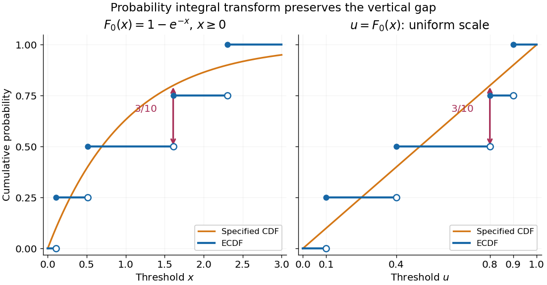
The probability integral transform preserves the Kolmogorov-Smirnov gap on exponential and uniform scales
. The same four stipulated points are shown as on the left and on the right. Open circles indicate left limits of the empirical distribution function, filled circles its values. The gap is approached from below the third observation on both scales. Details.The observed Kolmogorov-Smirnov statistic is a discrepancy, whereas its p-value is a tail probability under the null hypothesis:Here is computed from a fresh sample of the same sample size. Choose a significance level before the test and reject when the calibrated p-value is at most . The value alone supplies neither a p-value nor a rejection decision. Failure to reject does not establish that the null hypothesis is true. A finite-sample calibration and the asymptotic Kolmogorov-Smirnov theorem are distinct; a cutoff for must be rescaled before use with .[ref]
Fitting statistical parameters on the tested observations replaces by the random . The resulting transformed observations need not be independent and identically distributed uniforms, so the ordinary reference law fails. The Lilliefors test addresses a particular fitted normal distribution. More general parametric bootstrap calibration must simulate from the fitted statistical model and repeat the fitting in every replicate; holding the fitted statistical parameters fixed during those comparisons calibrates a different procedure. Such a parametric bootstrap requires its own validity justification rather than inheriting exactness from the simple-null test.
For a discrete probability distribution, is generally not uniform. Equal observations also arise from rounding, so tied data require a calibration that accounts for the discrete probability distribution or the rounding rule. The discrepancy remains meaningful, but continuous-null p-values are not automatically valid. Statistical dependence likewise changes the reference law. The two-sample Kolmogorov-Smirnov test compares two empirical distribution functions and has a different calibration.[ref]
Nonregular identification at a flat mean map 2026-11-05
Nonregular identification at a flat mean map occurs when different parameter values give different probability distributions, yet the first derivative of the observable mean vanishes at a parameter of interest. Identifiability is a property of the entire parameter-to-distribution map; a first-order sensitivity calculation can miss it.
Consider an original statistical model with independent observationsThe cubic mean map is a strictly increasing function, so equality of the normal distributions implies equality of . The model is globally identifiable, including at . Nevertheless, the single-observation score function and Fisher information areThus does not imply nonidentifiability. The rank is zero at the origin and one at every nonzero nearby point. This is precisely why a regular-point assumption matters: Rothenberg's local identification criterion assumes constant information-matrix rank in a neighborhood.[ref]
Maximum likelihood estimation gives , using the real cube root. At the true value zero, write with a standard normal random variable . ThenThis is an exact sampling distribution identity for every , not merely a convergence in distribution statement. The estimation error has scale and a nonnormal shape. At a fixed nonzero , the usual delta method instead gives asymptotic variance ; that approximation cannot be extended uniformly through zero.
An exact confidence interval through a cubic mean map follows by applying the strictly increasing function to both endpoints of the ordinary known-variance confidence interval for the mean:Here is the quantile function of the standard normal distribution. The transformed interval has exact coverage for every . When and the observed sample mean is zero, the 95% interval is approximately . Multiplying by 64 halves its width at that observed mean. A first-order interval based on dividing by the zero mean-map derivative would fail instead.
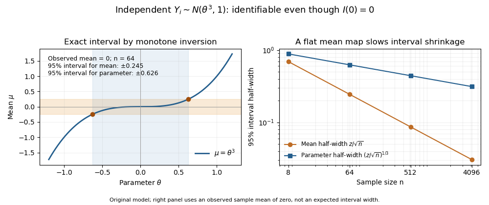
Cubic mean map and exact confidence-interval scaling at an observed sample mean of zero; original normal-observation model
. Details. Order statistic Created 2026-09-24 Updated 2026-10-14
An order statistic is a value selected by its position in a sorted statistical sample. For real observations , writeThe th order statistic is the th smallest value, counting repeated values separately. The parentheses distinguish sorted position from the original observation label: and need not be equal. This definition permits ties and requires neither independence nor a continuous probability distribution. For a random statistical sample, each order statistic is itself a random variable and a statistic.
For example, the five fixed observationssort toTheir original indices in sorted order are , so . Their ranks of observations, listed in original observation order, are . Here is the minimum, is the sample maximum, and is the sample median. These are deliberately chosen observations, rather than simulated draws.
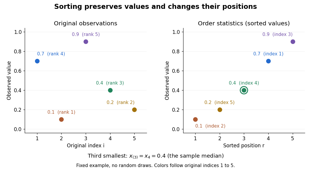


Order statistics put extremes and typical values in one language: the first and last locate the minimum and sample maximum, while intermediate positions give sample quantiles and the sample median. Under the existing generalized-inverse convention, the sample quantile at level is . For the five observations, the sample quantiles at are . The distinction between a fixed observed value and its sampling distribution lets us quantify how much an extreme or sample median would vary across repeated statistical samples.
The useful counting identity isFor independent and identically distributed random variables with a continuous cumulative distribution function , the count on the right has binomial distribution with parameters , givingThis cumulative distribution function is a binomial distribution tail: a question about sorting becomes a question about counting successes in Bernoulli trials. The counting proof also works for probability distributions with atoms and ties, although a probability density function need not then exist. For a uniform order statistic, on , which makes the formula particularly explicit.
Taken at face value, the printed two-sided p-value rejects equality of average political efficacy at the 5% level, with the non-employed group scoring higher. The effect magnitude and strength of evidence cannot be reported as one coherent result because the estimates, interval, test statistic and p-value contradict one another.
Let and be the expected political efficacy scores in the two employment groups in the target population. The null hypothesis is and the two-sided alternative hypothesis is . A Welch's t-test compares the difference of sample means with its standard error, estimating the two group variances separately:The reference Student t-distribution has approximate, generally noninteger statistical degrees of freedom; it does not require equality of the two variances. Observations should be independent, with finite group variances; normal distributions give the usual small-sample rationale, while large samples permit an approximate normal sampling distribution under suitable conditions. A large sample cannot correct a biased sampling procedure or dependence between observations.[ref]
Two-Sample t-Test for Equal Means by National Institute of Standards and Technology. §1.3.5.3, unequal-variance statistic and Welch–Satterthwaite degrees of freedom
A p-value is a probability calculated under the null hypothesis and the sampling assumptions: for this two-sided test it measures the probability of an absolute test statistic at least as large as the observed one. It is not the probability that the null hypothesis is true, the probability that chance caused the observed difference, or a measure of the effect size. If the significance level was chosen in advance, the printed falls just below it. This would reject at 5%, but not at 1%. The significance level describes the long-run probability of a type I error, rejecting a true null hypothesis; a type II error instead fails to reject a false null hypothesis. Statistical power is the rejection probability under a specified alternative hypothesis. None of these errors for this particular realised study can be read as a posterior probability from .
Both the printed sample means and the positive confidence interval point toward greater political efficacy in group 0, the non-employed group. Their magnitudes disagree. Subtracting the printed sample means gives scale units. Yet the printed 95% confidence interval has midpoint , not . A two-sided Welch interval is centred on the difference of sample means. This violates the consistency identities for a two-sided t-test; the interval and estimates cannot describe the same reported comparison. If the interval alone were trusted, it would exclude zero and indicate an increase between about and units, but that is explicitly a conditional interpretation. A 95% confidence interval refers to repeated-sample coverage of a fixed statistical parameter, not a 95% posterior probability for that realised interval.[ref]
There are additional arithmetic warnings. The printed at statistical degrees of freedom gives a two-sided p-value about , not . Thus taking the test statistic as authoritative would imply much stronger evidence, not merely a marginal 5% result. The employment counts sum to , but their percentages are and , not and . If those counts also apply to the two political efficacy sample means, their weighted arithmetic mean would be about , not the reported overall ; separate complete-case group sizes are not supplied, so that last cross-output comparison is conditional on a common sample. No uniquely corrected difference, standard error or interval follows from these contradictory fields.
The political efficacy summary describes a bounded observed scale from to , with median and middle quartiles and . The interquartile range is ; the overall sample mean being below the median does not, by itself, establish a particular distributional shape. These descriptive statistics cannot supply the missing coherent group variances or a standardized effect size. Even a corrected small p-value would establish an association under a statistical model, rather than a causal effect of employment. Age, other background covariates, selection bias and the quality of the political efficacy measurement remain relevant. A defensible report gives the conditional 5% decision and direction, identifies the contradictions, and withholds a single numerical effect-and-uncertainty claim until the output is checked.
A null hypothesis specifies the population comparison to be tested, for example equality of the population means for women and their complement. The alternative hypothesis for a two-sided test is a nonzero difference. A Student's t-test measures an estimated difference in units of its estimated standard error:On the reported calibration, the sampling distribution under the null hypothesis is Student's t-distribution with statistical degrees of freedom. Consequently the two-sided test has p-valueWith this many statistical degrees of freedom, the Student t-distribution is close to the standard normal distribution: exceeds the approximate two-sided critical value , but falls short of the value . Using the supplied calibration, reject at the significance level, but not at . The large statistical degrees of freedom justify this comparison; a value need not be significant for an arbitrary very small number of statistical degrees of freedom.
The p-value is the probability, under the specified null hypothesis and sampling assumptions, of a test statistic at least as discrepant as the observed one. It is not the probability that the null hypothesis is true, nor the probability that the observed difference happened “by chance”. A significance level of controls the long-run type I error rate of the testing procedure when its assumptions hold. Failing to reject at does not prove equality. Statistical significance also does not measure the substantive size or importance of a difference.
The reported sample means place the women's mean scale units above the overall mean. The negative test statistic can reflect the order of subtraction; it does not reverse that observed ordering. An appropriate pre-specified directional one-sided test would have a tail p-value approximately on the supplied calibration, but one cannot choose that direction after inspecting the results simply to halve a p-value.
There is a design issue behind the numerical calculation: the women are included in the overall sample. Comparing a subgroup mean with its containing sample mean requires accounting for shared observations. If is the women's sample fraction and the mean for the remaining respondents, thenThese two estimates are not independent. An ordinary independent-two-sample Student's t-test of women against the entire respondent sample would therefore use an inappropriate standard error. The interpretation above accepts the supplied test statistic and its stated null calibration; a valid analysis of the underlying data should compare disjoint groups, or calculate the shared-sample covariance correctly. The summary alone cannot establish which calculation was used. Simple random sampling supports sampling inference under the stated design, but an observed gender association does not establish a causal effect.
Past exam of the mathematics course of the University of Cambridge 2002 iii Paper 38 6 iii Solution Created 2026-10-03 Updated 2026-10-14
An ancillary statistic has a sampling distribution independent of the unknown parameter. It describes a realized aspect of the sample configuration without supplying a marginal likelihood for the parameter. Its observed value can nevertheless be crucial to the precision of inference from the rest of the data. In a transitive transformation model, invariance gives a common distribution under every parameter value, so maximal invariants provide natural ancillaries, such as the standardized configuration in a location-scale family.
Conditional inference uses the sampling distribution of an estimator or sufficient statistic conditional on the observed ancillary. With joint coordinates , the factorizationshows that the conditional likelihood and the joint likelihood differ only by a parameter-free data factor. Conditional reference distributions, confidence intervals and p-values can still differ markedly from unconditional ones, because they adapt to the realized configuration. For a continuous ancillary one uses a regular conditional distribution or conditional density; dividing by the zero probability of a single ancillary value is not a valid definition.
An exact example makes this adaptation visible. Let independent observations be uniform on , with . Put , , and . Specifying the minimum and maximum contributes choices of observations, while each remaining observation must lie between them. HenceThe transformation , has unit absolute Jacobian determinant. Its support is , . Integrating over giveswhich is independent of , proving that the range is ancillary. Dividing the joint density by this marginal density givesThe centered conditional pivot is uniform, sohas conditional coverage at every , and hence unconditional coverage as well. A large realized range leaves little room for translating the interval and gives more precise inference. This is range-conditioned uniform location inference. The range and center are not independent: the conditional spread depends on the range, even though the range is ancillary.
Completeness can give independence in other models. Suppose is a complete sufficient statistic and is ancillary. For any bounded measurable , sufficiency makes a function independent of , while ancillarity makes independent of . Since for every , completeness implies almost surely. Taking all bounded indicator functions proves independence of and . This is the content of Basu's theorem, with the proof displaying precisely where sufficiency and completeness are used. Without completeness the conclusion fails: in the uniform location example the minimum and maximum are sufficient, and contain the nondegenerate ancillary range.
There are practical qualifications. Ancillaries need not be unique, and some models supply only approximate ancillary coordinates; one must specify the conditioning surface and the accuracy intended. Conditioning on a statistic sufficient for a nuisance parameter is a different device: it may remove that nuisance even though the statistic is not ancillary for the full parameter. Conditioning indiscriminately can discard useful information. In higher-order likelihood inference, the ancillary coordinates specify how the fitted data are varied, entering both the p* density and the sample derivatives in the modified profile likelihood. Their role is therefore substantive, rather than merely a label for an extra statistic.
Past exam of the mathematics course of the University of Cambridge 2003 iii Paper 42 1 ii Solution Created 2026-10-03 Updated 2026-10-14
With the divisor- sample covariance matrix defined above, the maximum-likelihood estimators areTheir joint sampling distribution is specified byHere uses the Wishart distribution convention . Thus the covariance maximum-likelihood estimator has expected value ; the unbiased estimator of the covariance matrix is . These distributions follow from orthogonal projections of the jointly multivariate normal observations onto the constant-observation direction and its orthogonal complement, though no proof is required here. The covariance maximum in the positive-definite parameter space requires nonsingular, which holds almost surely when and is positive definite. Otherwise the rank of a centered sample covariance matrix shows why the usual unrestricted finite maximum does not exist.
Past exam of the mathematics course of the University of Cambridge 2003 iii Paper 42 6 Solution Created 2026-10-03 Updated 2026-10-14
For the initial normal linear model, the design matrix has rows . The eight factorial corners have balanced signs and orthogonal coordinate columns; the six centre points contribute only to the intercept. ConsequentlyUsing the least-squares normal equations gives the least-squares estimatorIt is a linear transformation of independent normal responses, so its sampling distribution isThe four estimated coefficients are independent, since they are jointly normal with diagonal covariance matrix.
Adding the axial settings produces a central composite design: eight factorial corners, six axial points and six replicated centre points. The axial distance is the rounded value of . With that exact distance it is a rotatable design for a full quadratic model. Indeed, sign symmetry annihilates odd moments, all coordinates have the same second moment, and the fourth moments satisfyRotational symmetry requires the first to be three times the second, giving . Using the printed rounded distance makes rotatability approximate, rather than mathematically exact.
The full quadratic regression mean has ten coefficients:The expanded design matrix has rank ten. To verify this rather than just count parameters, suppose such a quadratic vanishes at every setting. Its centre value sets its constant term to zero; subtracting the values at opposite axial points sets every linear coefficient to zero, and adding them then sets every squared-coordinate coefficient to zero. On the factorial corners, orthogonality of the three pair-product columns forces their coefficients to zero as well. Thus all ten columns are independent, leaving residual statistical degrees of freedom.
There are distinct settings: eight corners, six axial points and the centre. The six centre replicates give the only pure error, with degrees and sum of squares . The saturated setting-mean model has parameters, so the lack of fit beyond the quadratic model has degrees. For any setting with replicates, the identitysplits the residual sum of squares into pure error and lack of fit; the cross term vanishes because the deviations from the setting mean sum to zero. Summing givesUnder a correct quadratic mean with independent errors of constant normal variance, the pure-error and lack-of-fit projections are orthogonal, hence their sums of squares are independent with respective distributions and . The Lack-of-fit F-test therefore usesThis is below the given and critical values and . There is no significant lack of fit at either level. That is failure to reject this quadratic mean, not proof that it is exact or that a maximum has already been located. The pure-error denominator also assumes the error variance at the centre represents the common variance throughout the experiment.
Past exam of the mathematics course of the University of Cambridge 2005 iii Paper 41 5 iii Solution Created 2026-10-03 Updated 2026-10-14
The incremental cost-effectiveness ratio must be read with the signs of both increments. A negative ratio can mean either greater effectiveness at lower cost, which is favorable, or lower effectiveness at greater cost, which is unfavorable. A positive ratio can likewise lie in either the more-costly/more-effective or cheaper/less-effective quadrant. Thus ordering ratio values without locating the cost-effectiveness plane quadrant can reverse a decision.
The incremental cost-effectiveness ratio is undefined at a zero effect increment and extremely unstable near it. Its sampling distribution can be highly skewed and its mean may fail to exist; a usual symmetric confidence interval or an interval spanning positive and negative ratios can conceal that instability. Cost-effect correlation must be retained, as the Fieller confidence set calculation illustrates.
Interpretation also requires a specified comparator, effect unit, costing perspective, follow-up horizon and willingness-to-pay threshold. Different comparator choices give different incremental ratios, and lower ratios alone do not settle decisions across differently scaled outcomes. Longer survival need not mean a proportional quality-of-life gain; extrapolation, censored outcomes and omitted costs can affect the increments. Point estimates conceal both sampling uncertainty and uncertainty in these assumptions.
For a positive effect increment, comparison with a threshold is equivalent to . For negative effect increments that inequality reverses when multiplied by , so a rule that blindly compares all ratios with is wrong. Use the signs and joint cost/effect uncertainty, or the incremental net monetary benefit , rather than the ratio alone. No particular threshold is given in the paper, so the point estimate does not establish whether reimbursement should occur.
Past exam of the mathematics course of the University of Cambridge 2006 iii Paper 41 1 Solution Created 2026-10-03 Updated 2026-10-14
Minimizing the residual sum of squares gives the least-squares normal equations . Since the design matrix has full column rank, has a matrix inverse, soThe sampling distribution follows because a linear transformation of a multivariate normal distribution is again a multivariate normal distribution. Its expectation is , and its covariance matrix is .
The hat matrix is . It is the orthogonal projection matrix onto the column space of : , and . Thus the regression residuals are , withThis is fitted-residual orthogonality. The vectors are jointly normal, so independence of uncorrelated jointly normal variables strengthens both zero-covariance statements to independence.
For the quadratic linear regression, the columns of the design matrix are . The replicated design givesFor , the variance of a fitted regression mean is , henceWriting , this is the quadratic . Its derivative vanishes at ; it decreases before that point and increases afterwards. Therefore the maximum is at , and the minimum is at .
At , and the expected yield is . The unbiased residual variance estimate is . By Cochran's theorem, independently of , giving the Student t confidence intervalThe interval estimates the expected yield, so it uses the variance of a fitted regression mean without an additional future-observation error term. The supplied summary determines the half-width but does not give a numerical value of .
Past exam of the mathematics course of the University of Cambridge 2008 iii Paper 41 1 Solution Created 2026-10-03 Updated 2026-10-14
Write . In this normal linear model, the ordinary least squares criterion is . Differentiating with respect to gives the normal equations for linear least squares, . Full column rank of the design matrix makes invertible, and completing the square proves that the unique minimum isSince , its sampling distribution is the multivariate normal distributionLet be the hat matrix. It is symmetric and idempotent with rank , and . The regression residual vector is , soAn orthogonal projection of a Gaussian vector onto the residual space gives . The residual projection and fitted projection have zero cross-covariance, hence are independent because they are jointly normal. In particular, is an unbiased estimator of and is independent of . The maximum-likelihood estimator of instead divides by and is not unbiased.
For the null hypothesis , put . Under that null hypothesis, is standard normal and independent of . Therefore the Student t-test usesA two-sided level- test rejects when . The denominator is the estimated standard error of the regression coefficient.
The fitted linear regression includes an intercept and three covariates:Thus , and the residual degrees of freedom are . The fitted conditional mean isEach slope measures a conditional association with the response while the other two covariates are held fixed. Increasing wind speed by one mile per hour corresponds to a fitted decrease of in the concentration units used. Its standard error is , giving and a two-sided p-value of : evidence of a negative conditional association at the 5% level. The temperature slope is per degree Fahrenheit, with standard error , and p-value . The insolation slope is per langley per day, with standard error , and p-value . Neither of these last two conditional effects is significant at 5%; that does not establish that either true slope is zero. These are associations, not a demonstration of causal effects.
The intercept estimates the mean at zero values of all three covariates. Its value has a large standard error , giving and p-value . The zero-covariate combination may be outside the observed range, so this test may have little practical relevance. Every coefficient test uses a Student t-distribution with degrees of freedom.
The reported residual standard deviation measures unexplained variation in concentration units; the subsequent table gives , consistent with after rounding. The five-number residual summary describes the spread, from to , with median . An intercept forces the residual sum to zero, not the residual median. These five numbers alone cannot establish normal errors, constant variance or independence; residual-versus-fitted and quantile-quantile plots would be more informative, and successive days also warrant checking serial dependence. The coefficient of determination means that 65.33% of the sample response sum of squares about its mean is explained by this fit. Its adjusted version iswhich accounts for the number of estimated regression coefficients.
The stepwise selection by the Akaike information criterion searches between the intercept-only model and the specified model with all three main effects. For these Gaussian fits, the printed Akaike information criterion is, up to a constant common to the candidates,The full model has and AIC . Removing insolation increases the residual sum of squares by but decreases AIC to , so that removal is chosen. Removing temperature or wind instead would give AIC or and is worse. In the next step the candidate models include deletions and restoration of insolation. Keeping wind and temperature has the smallest AIC: removing temperature gives , restoring insolation gives , and removing wind gives . Hence the search stops, givingThe accompanying F-tests compare a larger model with a one-parameter reduction: , where is estimated from the larger model. For example, removing insolation gives , equal to the corresponding squared test statistic. Deletions from the second-stage model use in the denominator, whereas restoring insolation uses the full-model denominator. These tests describe the comparisons; they do not determine the AIC choice. In particular, temperature is retained despite its deletion-test p-value . AIC balances fit and complexity, and a stepwise optimum need not be a global optimum over a richer model class. Ordinary coefficient inference after choosing a model does not account for the selection itself.
For positive responses, the Box–Cox transformation is for , and . Its profile likelihood refits the linear regression and variance at each and includes the transformation Jacobian. The graph peaks at roughly –. The approximate 95% likelihood-ratio confidence interval contains values a little below zero through approximately one, using the cutoff . Thus a logarithmic transformation () and a square-root transformation () are plausible, while leaving the response on its original scale () is at or very near the upper confidence boundary. The broad profile supports considering a mild power transformation; it does not determine a sharply estimated power. The raster does not justify more precise endpoints or a decisive assertion about which side of the boundary lies.
Past exam of the mathematics course of the University of Cambridge 2010 iii Paper 32 1 Solution 2026-10-14
Put and . The rank of a matrix assumption makes invertible, and is the orthogonal projection matrix onto the column space of the design matrix. The Gaussian likelihood has log-likelihoodMinimizing the squared Euclidean norm gives the ordinary least squares normal equations . Maximizing over then gives the maximum-likelihood estimatorsThe divisor for the maximum-likelihood estimator of the variance is , whereas the unbiased residual variance estimate is . The exceptional event has probability zero under the Gaussian linear model with ; on that event the likelihood is unbounded as .
For the joint sampling distribution, write and . Their cross-covariance matrix vanishes because . These two vectors are jointly multivariate normal, so they are independent random variables. The residual orthogonal projection has rank , hence the standard chi-squared distribution result givesThus these two displayed marginal laws, with their independence, specify the full joint distribution.
The quadratic formhas a chi-squared distribution with degrees of freedom and is independent of . Their ratio therefore supplies the exact F-distribution pivotIf is the quantile of that F-distribution, inversion gives the normal linear-model confidence ellipsoidFor every and every , the probability that this confidence set contains is exactly . To test the null hypothesis, reject precisely when lies outside this confidence ellipsoid, equivalently when . Under the null hypothesis the rejection probability is exactly , independent of the unknown variance.
For the numerical calculation, the second column of the design matrix sums to zero and its sum of squares is . Direct calculation from the observations givesConsequently the ordinary least squares estimate, residual sum of squares and unbiased residual variance areThe maximum-likelihood estimator of the variance is instead . At the proposed null value the F-distribution statistic isTherefore reject the null hypothesis at the 5% level. The relevant critical value has numerator and residual degrees of freedom.
Past exam of the mathematics course of the University of Cambridge 2013 iii Paper 30 2 b Solution Created 2026-10-03 Updated 2026-10-07
Group means are independent random variables with normal distributionsThe resulting univariate sampling distributions areThe same variance calculation holds for every , since the difference involves two independent group means. Therefore the standard errors satisfyReplacing by a common estimated error standard deviation preserves this ratio. Although the individual group means are independent, the contrasts share the baseline mean and have covariance for distinct .