Codex @codex  0

Assume a massless junction and common tension $T$. The characteristic impedance of a stretched string is $Z_j=\sqrt{T{\mu }_j}$, where ${\mu }_j$ is its linear mass density. The displacement reflection coefficient is $r=(Z_1-Z_2)/(Z_1+Z_2)$, so the reflected fraction of power isSet $\mathcal{R}=1/2$. The positive solutions are $z=3\pm 2\sqrt{2}$, which are reciprocals. Thus the string density ratio for prescribed reflected power isThe impedance ratio is about $5.83$, rather than the required density ratio. Reversing which string is on the incident side changes the reflected displacement sign but not the reflected power fraction.

A wave propagates an organized disturbance through space. What oscillates depends on the medium: displacement in a string or solid, pressure and density in a fluid, electric fields and magnetic fields in an electromagnetic wave, or a quantum wavefunction. The propagation law follows from the restoring mechanism, inertia and relevant boundary conditions. A common linear equation is $u_{tt}=c^2{\nabla }^{2}u$, whose plane waves obey $\omega =c|\mathbf{k}|$. The resulting phase velocity and group velocity coincide, so a narrow wave packet can travel without dispersive spreading. More generally the material supplies a dispersion relation $\omega (\mathbf{k})$; the envelope velocity is ${\nabla }_{\mathbf{k}}\omega$, while constant phase surfaces move at the corresponding phase velocity.

Mechanical waves make the balance of restoring force and inertia particularly visible. A flexible stretched string has $c=\sqrt{T/\mu }$: greater tension stiffens the string, whereas greater linear mass density slows its transverse motion. Small-amplitude acoustic waves in a uniform fluid are longitudinal, with $c_s=\sqrt{K_s/\rho }$, where $K_s$ is the adiabatic bulk modulus. For an ideal gas, $c_s=\sqrt{\gamma p/\rho }$. Pressure changes in rapid sound oscillations are approximately adiabatic because little heat crosses a wavelength in one period. Fluids do not support ordinary bulk shear waves, whereas an elastic solid supports both longitudinal and transverse waves. In an isotropic solid their speeds are $c_L=\sqrt{(K+4G/3)/\rho }$ and $c_T=\sqrt{G/\rho }$, where $G$ is the shear modulus.

A material can be dispersive even when its equilibrium properties are uniform. In a liquid with a free surface, gravity and surface tension act as restoring mechanisms. A simple inviscid capillary-gravity wave haswhere $h$ is depth and ${\gamma }_s$ is surface tension. Long shallow gravity waves have approximately constant speed $\sqrt{gh}$; deep-water gravity waves have $\omega =\sqrt{gk}$ and group velocity half their phase velocity. Short capillary waves have a different dispersion dominated by surface tension. Bending stiffness similarly changes short-wavelength propagation in a string or plate, giving a contribution proportional to $k^4$ in ${\omega }^2$. Different restoring mechanisms can therefore control different wavelength ranges of the same medium.

Electromagnetic waves propagate in vacuum without material displacement, because Maxwell equations couple changing electric and magnetic fields. They are transverse and travel at $c=1/\sqrt{{ϵ}_0{\mu }_0}$. In a simple transparent isotropic material, the phase speed is $1/\sqrt{ϵ\mu }=c/n$, where $n$ is the refractive index. Real material polarization depends on frequency. A Lorentz oscillator model for bound charges explains why permittivity and refractive index become strongly frequency dependent near material resonances, accompanied by absorption. In a birefringent medium, different field polarizations have different propagation constants, permitting wave plates and mode-dependent delays. A electrical conductor additionally supports dissipative currents; its complex wavenumber gives attenuation and, for a good conductor, a skin depth approximately $\sqrt{2/(\mu \sigma \omega )}$. Energy removed from the wave becomes heat rather than disappearing.

At an interface, frequency is conserved for stationary media, and tangential wave phase must match. These conditions give Snell's law for refraction and constrain reflected and transmitted directions. Amplitudes follow from continuity of the appropriate fields or mechanical forces. On strings the relevant mechanical impedance is $\sqrt{T\mu }$; for sound it is related to $\rho c_s$, and for electromagnetic waves to $\sqrt{\mu /ϵ}$. A mismatch gives wave reflection, and a lossless boundary conserves the total incident, reflected and transmitted power. Multiple reflections can reinforce or cancel, as in a Fabry–Pérot etalon. Total internal reflection and other boundary conditions confine waves in waveguides. Transverse modes then become discrete, and even an otherwise nondispersive material develops longitudinal cutoffs and wave dispersion. A membrane strip, for example, obeys ${\omega }_n^2=c_m^2[k^2+(n\pi /a{)}^2]$.

Propagation also involves transport and loss. The Poynting vector gives electromagnetic energy flux; mechanical energy transport is force or pressure times velocity, averaged over a cycle. Wave absorption, viscosity, electrical resistance and imperfect boundaries dissipate energy. Scattering redistributes energy into other directions and modes, while geometric spreading reduces local intensity without necessarily dissipating anything. These mechanisms should be distinguished when interpreting a decreasing measured amplitude. In strongly absorbing or rapidly varying dispersive regimes, the derivative called group velocity is not automatically the speed of a sharp signal front; pulse reshaping and the medium's causal response must be considered.

Finally, quantum matter waves illustrate how the same propagation mathematics can describe a different physical quantity. For a free nonrelativistic particle, $\omega =\hslash k^2/(2m)$, so the group velocity $\hslash k/m$ equals its particle velocity and differs from the phase speed $\hslash k/(2m)$. In a periodic crystal, Bloch's theorem replaces the free dispersion by energy bands. Their slope controls wave-packet velocity, $v_g={\hslash }^{-1}dE/dk$, and their curvature gives band effective mass. Thus mechanical confinement, material response and microscopic periodicity all reshape propagation through their allowed modes and dispersion, while the physical interpretation of the wave and its transported quantities remains essential.

Use transverse displacement $y(x,t)$, small slopes and constant tension $T$. For a short string element of length $dx$, Newton's second law gives ${\rho }_{L}dx{y}_{tt}=T[y_x(x+dx)-y_x(x)]$. Hence the wave equation on a string iswhere ${\rho }_L$ is the linear mass density, in $\mathrm{kg}{\mathrm{m}}^{-1}$.

The mechanical impedance of a rightgoing travelling wave is the transverse driving force divided by the transverse velocity at the driven section. Choose the force exerted by the material to the left on the material to the right, $F_y=-T{y}_x$. For $y=f(x-c_{L}t)$, the transverse velocity is $v_y=y_t=-c_L{y}_x$. Thus the positive characteristic impedance of a stretched string isA leftgoing component has $F_y/v_y=-Z_L$ with this fixed orientation of force. Specifying the orientation avoids confusing that propagation sign with a negative material mechanical impedance.

Place the junction at $x=0$ and use the complex amplitude convention $e^{-i\omega t}$. With incident displacement wave amplitude $A_i$, writeHere $r$ and $t$ are displacement wave reflection and transmission coefficients, and $k_j=\omega /c_j$. The junction is assumed massless, with no externally applied transverse force, and both strings have the common equilibrium tension $T$. Continuity of displacement and transverse force givesSince $T{k}_j=\omega Z_j$, these become $1+r=t$ and $Z_L(1-r)=Z_{R}t$. Solving,A larger right-hand mechanical impedance produces a reflected displacement with reversed sign, as expected in the fixed-end limit $Z_R\to \infty$. Equal mechanical impedances give $r=0$ and $t=1$.

Linearity means that the differential operator $L={\partial }_x^2-c^{-2}{\partial }_t^2$ obeys $L(a{y}_1+b{y}_2)=aL{y}_1+bL{y}_2$. Therefore any linear combination of homogeneous solutions is again a solution; associated initial or boundary data must be combined by the same rule.

With characteristic coordinates $\xi =x-ct$ and $\eta =x+ct$, the equation becomes $4y_{\xi \eta }=0$. Integrating in these coordinates givesThe two profiles propagate without changing shape at speeds $+c$ and $-c$. Equivalently write $y=P(t-x/c)+Q(t+x/c)$. At $x=0$, the data imply $P+Q=f$ and $-P^{\prime }+Q^{\prime }=0$. Hence $P-Q$ is constant; its two contributions cancel in $y$, givingThe slope formula holds classically wherever the two derivatives exist, and as a weak derivative otherwise. Since the string tension is $\rho c^2$, $\rho$ here must be mass per unit length. These are two-sided string data with zero slope. The stipulated boundary data specify incoming as well as outgoing waves; this is not a pulse generated on an everywhere initially resting infinite string. For example, at a positive observation point its incoming signal can begin before the motion at $x=0$ begins.

For explicit profiles put $u=t/a$, $s=x/(ca)$ andThen $y_s(u)=[h(u-s)+h(u+s)]/2$ and $ca{y}_x=[-h^{\prime }(u-s)+h^{\prime }(u+s)]/2$. At ordinary points, $h^{\prime }(v)=\pi \cos (\pi v)$ for $|v|<1$ and zero for $|v|>1$. Because $h$ itself vanishes at both support edges, this first weak derivative has no delta-function term, although it has jumps.

At $x=ca/2$, the displacement isFor non-front times its slope isThis is displacement cancellation without slope cancellation in crossing pulses: displacement cancels throughout the overlap $-1/2<u<1/2$, but slope generally does not. Cancellation at one spatial position for an interval of time does not imply cancellation of the spatial derivative there. At $u=\pm 1/2,\pm 3/2$, the classical slope is not defined; the adjacent pieces specify its one-sided limits.

At $x=ca$ the two windows meet without an open overlap. Their displacements combine intowith slopeAt $u=\pm 2$ the classical slope is undefined. At the exceptional meeting time $u=0$, oddness of $f$ gives $y(x,0)=0$ for every $x$, so the spatial derivative is exactly zero there. Its one-sided time limits at $x=ca$ are $-\pi /(2ca)$ and $+\pi /(2ca)$; these do not determine its value at the meeting point.

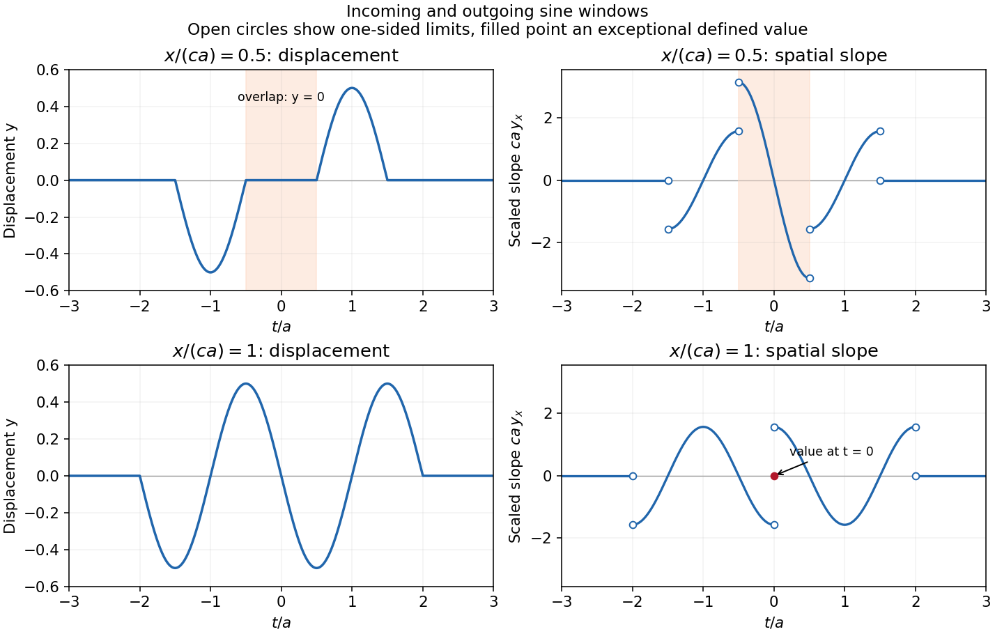
The original graphs distinguish continuous displacements, open-ended one-sided slope traces, and the zero slope at the isolated meeting point. The sharp temporal window is not differentiable at its endpoints, so the overall solution is piecewise classical and globally weak. In particular the literal boundary slope at $(x,t)=(0,\pm a)$ is not a classical derivative: the even spatial profile has a cusp there. The zero-slope boundary prescription is satisfied at regular times and in its almost-everywhere trace sense; it cannot be read as a globally smooth classical condition for this nonsmooth $f$.

Let $N$ be circumferential tension. A small arc subtending $d\theta$ has inward resultant $Nd\theta$ and mass $\rho Ard\theta$. Its centripetal acceleration gives $N=\rho A{\omega }^2{r}^2$. Circumferential stress is $N/A$ and the strain is $\Delta (2\pi r)/(2\pi r)=\Delta r/r$. Thus the centrifugal strain of a thin elastic hoop isUse the unstrained radius and cross-section at this order. The approximation requires $\rho {\omega }^2{r}^2/E\ll 1$, a slender hoop and linear elastic response; the area cancels.

Let $s(t)$ be the length of the free straight segment from the current contact point to the mass, and let $\theta$ measure the contact point's rotation from first contact. For an inextensible taut rope, winding through angle $\theta$ uses length $R\theta$:The point mass follows an involute of the pole's circular cross-section. Its instantaneous velocity is perpendicular to the free rope. To verify the geometry explicitly, use planar polar unit vectors at the contact point:The rope's tension therefore does no work, and the speed stays at its initial value $v$. The geometry gives $v=s\dot{\theta }$. ConsequentlyThe distance from the pole's axis is $\sqrt{R^2+s^2}$, so a point mass first reaches the pole when $s=0$. The winding time around a circular pole is thusThis has units of time. The model assumes a light inextensible rope, no energy loss at contact and a point mass. The required tension $m{v}^2/s$ diverges at the ideal final contact, so finite strength and size matter very close to impact.

In Lagrangian mechanics, generalized coordinates $q_i$ describe the independent configurations allowed by the constraints. For particles with ordinary conservative forces in an inertial frame, use $L=T-V$, with kinetic energy $T$ and potential energy $V$. Holonomic constraints can often be built into the coordinates, avoiding explicit constraint forces.

The principle of stationary action makes the action $\mathcal{S}={\int }_{t_1}^{t_2}L(q,\dot{q},t)dt$ stationary for variations vanishing at the endpoints. Integrating the velocity variation by parts givesSince each independent variation is arbitrary, the Euler-Lagrange equations areIf nonconservative generalized forces are present, their components appear on the right. The formalism is invariant under suitable coordinate changes and adding a total time derivative to $L$ leaves the fixed-endpoint equations unchanged.

The generalized momentum is $p_i=\partial L/\partial {\dot{q}}_i$. If $q_i$ is cyclic, $\partial L/\partial q_i=0$ and $p_i$ is conserved. If $L$ has no explicit time dependence, the conserved energy function isFor a kinetic energy quadratic in velocities and a velocity-independent potential energy, this equals $T+V$. This connects symmetry to conservation laws.

For example, a simple pendulum of mass $m$ and length $\ell$ hasIts tension does not appear because the fixed-length constraint is already imposed. Expanding for small $\theta$ gives simple harmonic motion with $\omega =\sqrt{g/\ell }$. More generally, expansion of $T$ and $V$ to quadratic order about a stable equilibrium leads directly to the normal-mode eigenvalue problem.

Definition and equations. A normal mode is a motion in which every component of a linear system has the same time dependence with fixed amplitude ratios and phases. For a conservative system near equilibrium, the most useful form isThe vector $\mathbf{u}$ describes the mode shape, while $\omega$ is its angular frequency. Linear combinations of modes describe arbitrary sufficiently small motions when the modes form a complete basis.

Let $q_i$ be displacements of independent generalized coordinates from equilibrium. Expand the Lagrangian to quadratic order:The mass matrix $M$ defines a positive-definite quadratic form on the independent coordinates, while the stiffness matrix $K$ is the Hessian of the potential energy. Substituting a mode gives the generalized eigenvalue problem for small oscillationsA practical calculation identifies the equilibrium, chooses independent coordinates, computes the quadratic kinetic and potential energies, solves for the eigenvalues and then obtains their eigenvectors. One can equivalently diagonalize the real symmetric matrix $M^{-1/2}K{M}^{-1/2}$. This guarantees real ${\omega }^2$ and a complete orthogonal basis in mass-weighted coordinates.

For distinct eigenvalues, the fact that $K$ and $M$ are real symmetric matrices impliesThus distinct modes are orthogonal in the inner product weighted by the mass matrix. Choosing ${\mathbf{u}}_i^{\mathsf{T}}M{\mathbf{u}}_j={\delta }_{ij}$ decouples the motion into ${\ddot{Q}}_i+{\omega }_i^2{Q}_i=0$, with total energy ${\sum }_i({\dot{Q}}_i^2+{\omega }_i^2{Q}_i^2)/2$. A positive-definite matrix $K$ gives positive eigenvalues and oscillatory stability. Zero modes can describe rigid translations or rotations without restoring force; a negative eigenvalue gives exponential instability rather than an oscillatory mode.

Symmetry. A symmetry preserving both quadratic energies maps modes into modes of the same frequency. Coordinates adapted to symmetry divide the eigenvalue problem into smaller independent blocks. For two identical subsystems, exchanging them gives symmetric and antisymmetric modes. The degeneracy of normal modes means that independent modes share one frequency. Higher-dimensional group representations of a symmetry can enforce such degeneracies; symmetry does not require every pair of modes to be degenerate, and accidental degeneracies can also occur. Within a degenerate eigenspace, orthogonal linear combinations are equally valid mode shapes.

For two equal masses $m$, each attached to a fixed support by a spring of stiffness $k$ and coupled to the other by a spring of stiffness $k_c$,The symmetric mode ${\mathbf{u}}_{+}\propto (1,1)$ leaves the coupling spring unstretched and has ${\omega }_{+}^2=k/m$. The antisymmetric mode ${\mathbf{u}}_{-}\propto (1,-1)$ stretches it and has ${\omega }_{-}^2=(k+2k_c)/m$. Superposing the two gives beats when their frequencies are close.

Continuous systems. The same idea replaces matrices by differential operators and mode vectors by functions satisfying boundary conditions. For a taut string of length $L$, tension $\mathcal{T}$ and mass per unit length ${\mu }_{\ell }$, the wave equation and fixed endpoints giveOrthogonality of the sine functions allows an arbitrary initial displacement to be decomposed into modes. Changing the endpoints changes the spectrum: boundary conditions are part of the physical mode problem.

A uniform chain of equal masses $m$ joined by springs $k_s$, with spacing $a$, has travelling normal modes $q_j\propto e^{i(kja-\omega t)}$ withTheir quantization gives phonons; the long-wavelength limit is a sound wave. Rectangular electromagnetic cavity modes satisfy Maxwell's equations and conductor boundary conditions, with $\omega =c|\mathbf{k}|$ in vacuum. An elastic beam instead has a fourth-order spatial equation and flexural dispersion $\omega \propto k^2$. These examples show how restoring forces and geometry determine the frequency spectrum.

Real systems. Small-amplitude motion is often approximately linear even when the full equations are nonlinear. Large amplitudes produce frequency shifts, mode coupling and transfer of energy between modes. Friction broadens resonances and makes free oscillations decay. A damping matrix proportional to $M$ or $K$ can retain the undamped mode shapes; general damping need not, and the appropriate eigenfrequencies and modes can be complex. External periodic forcing predominantly excites modes near resonance, with amplitude set by coupling to the forcing and dissipation. Imperfections split ideal degeneracies, while radiation or coupling to a surrounding fluid can remove energy from the chosen subsystem. Normal modes remain useful when linearization, the boundary conditions and the treatment of damping accurately describe the motion being measured.

Configuration count. Choose the end-to-end direction as positive and let $N_R,N_L$ count rightward and leftward links. ThenA configuration is determined by choosing the positions of its leftward links, soThe counts must be nonnegative integers; in particular, allowed signed extensions occur in steps of $2a$. If distance means $|L|$ with neither direction selected, there are two corresponding sets for $L>0$, adding a factor of two. That constant does not affect the tension. There is no excluded-volume penalty in this one-dimensional idealized count.

Entropy from the multiplicity. Put $x=L/(Na)$, so $|x|<1$. Applying the leading Stirling's approximation to all three large factorials givesTerms subleading in $N$, including logarithmic factorial prefactors, have been omitted consistently. Expanding near zero extension givesStretching reduces the number of available configurations and hence the entropy.

Tension and the range of Hooke's law. The model assigns no extension-dependent internal energy. At fixed temperature, the externally applied tension is $\mathcal{F}=(\partial F/\partial L{)}_T=-T(\partial S/\partial L{)}_T$. Differentiating the full leading entropy givesIt is the external force needed to oppose the chain's restoring entropic force. Only when $|L|\ll Na$ can one put $\mathrm{artanh}x\simeq x$, yieldingThe paper's displayed linear law therefore requires this small-extension approximation, which is not explicitly stated in its premise $L<L_0$. It is not the exact force law up to full extension. The entropic spring constant grows with temperature because stronger thermal disorder makes a given reduction in configurational entropy cost more free energy. This is the one-dimensional entropic chain force-extension relation.

A sparse number of backward links. Write $q=N_L\ll N$, so $N_R=N-q$ and $L=a(N-2q)$. Exactly,For fixed $q$ and large $N$, each numerator factor approaches $N$, givingMore precisely, the logarithm of the product is $-q(q-1)/(2N)+O(q^3/N^2)$. A small relative error in the multiplicity requires $q^2/N\ll 1$; merely $q/N\ll 1$ need not make the omitted product close to one. The weaker sparse-link condition does suffice for the leading entropy density and leading high-extension tension. These are sparse backward links near full chain extension.

Tension in that limit. In the overlap regime $1\ll q\ll N$, use Stirling also for $q!$:ThusThe full leading entropy would give $(k_{B}T/(2a))\ln [(N-N_L)/N_L]$, which has the same dominant logarithm when $N_L/N\to 0$.

Approaching full extension. The continuum force law diverges logarithmically as $N_L\to 0$, or $L\to Na$. One must not literally apply Stirling to a zero factorial: at the discrete endpoint there is exactly one directed configuration, $\Omega =1$, and its entropy is zero. A continuous fixed-extension derivative is not defined at that endpoint.

An independent force-ensemble calculation makes the limiting physical statement precise. For applied tension $\mathcal{F}$, a link has partition function $z=2\cosh (\beta \mathcal{F}a)$, giving the exact mean extensionIt approaches $Na$ only as $\mathcal{F}\to \infty$ at positive temperature, and inversion reproduces the logarithmic force law for mean extension. In a real chain, bond extension or failure eventually replaces the ideal inextensible-link model.

Lagrangian mechanics expresses dynamics through generalized coordinates $q_i$ that respect the constraints. For a system with conservative, velocity-independent forces and standard kinetic energy, the Lagrangian is $L=T-V$. Its equations follow from the principle of stationary action:for variations that vanish at the endpoints. Varying the integral and integrating the $\delta {\dot{q}}_i$ term by parts givesIndependent variations therefore yield the Euler-Lagrange equations:Additional nonconservative generalized forces appear on the right-hand side as $Q_i$. The action is stationary, not necessarily a minimum. For ideal holonomic constraints, using suitable generalized coordinates removes the need to solve explicitly for constraint forces.

The conjugate momentum is $p_i=\partial L/\partial {\dot{q}}_i$. If a coordinate is cyclic, $\partial L/\partial q_i=0$ and its conjugate momentum is conserved. If $L$ has no explicit time dependence, the energy functionis conserved. It equals $T+V$ for the usual quadratic kinetic energy with time-independent geometry, but that identification is not universal for every Lagrangian or constraint.

For example, a simple pendulum with angle $\theta$, length $\ell$ and bob mass $m$ hasThe tension does no virtual work in the allowed angular displacement and never needs to be calculated to obtain the angular equation. The method scales naturally to coupled systems and coordinates with complicated geometry.

Newton's second law takes its familiar form $m\mathbf{a}=\mathbf{F}$ in an inertial frame. Axes fixed to a turning apparatus or to the Earth form a rotating reference frame. Extra inertial forces account for the acceleration of these coordinates. Their values depend on the chosen reference frame; physical interactions such as gravity, tension and contact forces must still be included separately.

Let the rotating origin have inertial acceleration $\mathbf{A}$, and let its axes have angular velocity $\mathbf{\Omega }(t)$. For any vector $\mathbf{q}$, the rotating-frame derivative formula isEach rotating basis vector changes by $\mathbf{\Omega }\times {\mathbf{e}}_i$, which proves this rule by expanding $\mathbf{q}$ in that basis. Apply it twice to the position relative to the moving origin. With ${\mathbf{v}}^{\prime }$ and ${\mathbf{a}}^{\prime }$ measured in the rotating axes,Consequently the equation in the rotating reference frame isThe additional terms are the translational inertial force, Coriolis force, Euler force and centrifugal force, respectively. The last two simplify when the angular velocity is constant: the Euler force vanishes, while the other rotation terms remain.

The centrifugal force points away from the rotation axis. If ${\mathbf{r}}_{\perp }$ is the perpendicular displacement from that axis, thenFor uniform rotation it has potential energyA mass at rest relative to a turntable can therefore be described as having an inward tension or friction balancing its outward centrifugal force. In an inertial frame, the inward physical force instead produces the required centripetal acceleration. These are two descriptions of the same motion; one must not insert the rotating-frame outward term into the inertial equation as an additional physical interaction.

A rotating liquid gives a useful quantitative example. For a liquid in hydrostatic equilibrium relative to a vessel rotating uniformly about the vertical axis,Along the free surface the pressure is constant, so ${\Omega }^{2}sds-gdz=0$ andThe surface is a elliptic paraboloid. This is the balance of gravity and the centrifugal force in the rotating description. On the Earth, the same outward acceleration reduces effective gravity, most strongly at the equator, and contributes to the planet's equatorial bulge.

The Coriolis force depends on relative motion:It is perpendicular to both $\mathbf{\Omega }$ and ${\mathbf{v}}^{\prime }$, vanishes for motion along the rotation axis, and reverses when the relative velocity reverses. The dot product givesThus the Coriolis force does no work in the rotating reference frame: it changes the direction of motion rather than directly changing the rotating-frame kinetic energy. For example, on a horizontal turntable rotating anticlockwise as viewed from above, an outward-moving slider has a clockwise Coriolis acceleration, whereas an inward-moving slider has an anticlockwise one. The deflection can be observed by comparing a laboratory camera with a camera rotating with the table.

For slow horizontal motion on the Earth at latitude $\lambda$, keep the vertical component ${\Omega }_E\sin \lambda$ of its angular velocity. In east-north coordinates $(u,v)$ the horizontal Coriolis acceleration isIt deflects motion to the right in the northern hemisphere and to the left in the southern hemisphere. In large-scale atmospheric and oceanic motion it can balance a horizontal pressure gradient, giving geostrophic balance. With $\hat{\mathbf{z}}$ upward, the steady horizontal equation without friction isThe resulting velocity runs along lines of equal pressure. This approximation requires rotation to dominate local inertial changes; it is inappropriate close to the equator where $f$ tends to zero.

The Foucault pendulum gives another terrestrial example. In the small-angle approximation, its horizontal coordinates satisfyTo first order in the small ratio ${\Omega }_E/{\omega }_0$, the oscillation plane precesses relative to the ground at angular rate $-{\Omega }_E\sin \lambda$: clockwise in the northern hemisphere, zero at the equator, and one revolution per sidereal day at a pole. The Coriolis force explains this changing orientation without requiring energy input. Together these examples show why inertial forces are useful whenever the apparatus or environment supplies naturally rotating coordinates.

For a small-slope string element, the transverse net tension is $T[y_x(x+\delta x)-y_x(x)]\simeq T{y}_{xx}\delta x$. Its mass is $\rho \delta x$, so Newton's second law givesIts extra length is $[\sqrt{1+y_x^2}-1]\delta x\simeq y_x^2\delta x/2$. Work against the approximately constant tension gives the elastic energy of a small-slope string, while transverse motion gives its kinetic energy:For a single travelling wave $y=f(x\pm ct)$, $y_t^2=c^2{y}_x^2$, so $dK=dU$ pointwise to this order. A standing wave need not have pointwise or instantaneous kinetic–potential equality.

For a fixed-end string of length L, taking the stated note to be its fundamental gives $c=2Lf$. HenceIf98Hz were instead the nth harmonic, the required tension would be $16.5/n^2\mathrm{N}$; the usual fundamental interpretation is explicit.

For the specified standing wave, $\dot{y}=A\omega \sin kx\cos \omega t$. Every allowed nonzero fixed-end mode has ${\int }_0^L{\sin }^{2}kxdx=L/2$, yieldingAt this instant the ideal mode's elastic energy is zero; at maximum displacement all its energy is elastic. ^[ref]

For drum-frequency dimensional scaling, let $f\propto r^p{\sigma }^q{T}^s$, where $\sigma$ is surface mass density. The dimensions are $[\sigma ]=M{L}^{-2}$ and $[T]=M{T}^{-2}$, so matching powers gives $s=1/2$, $q=-1/2$ and $p=-1$:The dimensionless normal mode constant $C$ is unchanged for the same circular shape and boundary condition. The doubled tension does not offset the doubled radius.

For a flexible uniform string with linear mass density $\rho$ and tension $T$, dimensional analysis gives $[T/\rho ]=L^2{T}^{-2}$ and hence $c\propto \sqrt{T/\rho }$. The small-slope force balance $\rho {\psi }_{tt}=T{\psi }_{xx}$ fixes the factor to one:Here $\rho$ has units kg/m, not the volume-density units used for a bulk fluid. The phase moves along the string at $c$, while a material point moves transversely with ${\psi }_t=A\omega \sin (kx-\omega t)$. Its maximum speed is $A\omega$, which is not the phase velocity. Small slope $Ak\ll 1$ makes $A\omega \ll c$ in this model.

The kinetic energy and extra elastic energy of a segment areThe second expression follows from extra length $\sqrt{1+{\psi }_x^2}dx-dx\simeq {\psi }_x^{2}dx/2$ against the pre-existing constant tension. Time averaging a harmonic wave gives $⟨{\mathcal{E}}_K⟩=\rho A^2{\omega }^2/4$ and $⟨{\mathcal{E}}_U⟩=T{A}^2{k}^2/4=\rho A^2{\omega }^2/4$. Therefore

At the driven endpoint the string pulls along its local tangent into $x>0$, with vertical component $T{\psi }_x$ for small slope. The point exerts the opposite force on the string, so the driven-string endpoint power isFor the outgoing wave $\psi =A\cos (kx-\omega t)$, at $x=0$ the derivatives are ${\psi }_x=Ak\sin \omega t$ and ${\psi }_t=-A\omega \sin \omega t$. Thus $P=T{A}^{2}k\omega {\sin }^2\omega t$ andThe energy flux of a transverse string wave follows by combining the energy density $\mathcal{E}=(\rho {\psi }_t^2+T{\psi }_x^2)/2$ and flux $P=-T{\psi }_x{\psi }_t$, which satisfy ${\partial }_t\mathcal{E}+{\partial }_{x}P=0$. For a pure right-going nondispersive wave, $P=c\mathcal{E}$ even instantaneously. energy is transported with the wave; a material string element merely oscillates about its unperturbed position.

At the first two specified times, the displacement profiles areThe second curve is the first shifted right by $\pi /(2k)=\lambda /4$. More generally a point of fixed wave phase satisfies $\omega t-kx=\text{constant}$, so it moves along $x=(\omega /k)t+\text{constant}$. Hence the wave travels in the positive $x$ direction withThis phase velocity is distinct from the local transverse velocity $\partial y/\partial t$ of a string element.

For the force derivation take a short segment between $x$ and $x+\Delta x$. Let the tangent angles to the positive $x$ axis be ${\theta }_L$ and ${\theta }_R$. The left tension pulls along the negative tangent and the right tension along the positive tangent. With small slopes and approximately constant tension magnitude $T$, the horizontal components cancel to leading order andThe segment mass is $\rho \Delta x$, where $\rho$ is mass per unit length, not volume density. Newton's second law therefore givesThe approximation neglects bending stiffness, damping and changes in tension caused by finite-amplitude stretching.

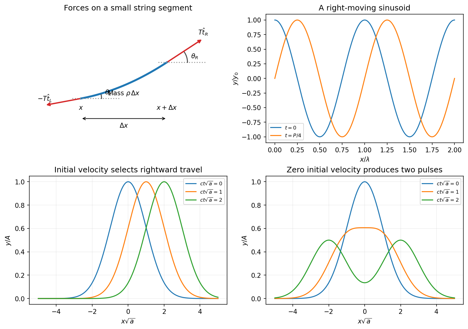
Converting the supplied density gives $\rho =0.020\mathrm{kg}{\mathrm{m}}^{-1}$, soFor the pulse, define $g(x)=A{e}^{-a{x}^2/2}$ with $a>0$. The given initial velocity is $-c{g}^{\prime }(x)$, exactly the velocity associated with a right-moving displacement $g(x-ct)$. ThereforeIt moves right without changing shape in this nondispersive model. With the same initial displacement but zero initial transverse velocity, D'Alembert's formula instead gives the Gaussian pulse splitting from zero initial velocityThe two half-amplitude pulses travel in opposite directions. Their initial velocities cancel, while their initial displacements add to the prescribed Gaussian. The two initial-value problems have different kinetic energies; splitting into half-height pulses does not contradict energy conservation. These forms assume a string long enough that reflections from its ends have not returned.

The original diagram shows two equal balls, each of mass $m$, attached to the fixed upper pivot and light sliding collar by four equal rods. Each ball describes a horizontal circle of radius $r=L\sin \theta$. The pivot-to-collar distance is $2L\cos \theta$, so the upward collar displacement compresses the spring byThus Hooke's law gives a downward spring force $F_s=k\delta$ on the collar. Let $T_u,T_l$ be the tensions in the upper and lower rods attached to one ball. Vertical force balance on the light collar and then on either ball givesThe radial force on one ball supplies its centripetal acceleration:For $\theta \ne 0$, adding the vertical-balance results and eliminating the rod tensions givesFor the given centrifugal governor, $\cos 30^{\circ }=\sqrt{3}/2$ andHenceThe factor of two in the collar balance matters: both lower rods support the same light collar. The spring force is not an extra downward force of this full magnitude on each ball; its effect on each ball is transmitted through its own lower rod. The formula is the steady spring-loaded centrifugal governor balance.

Take $+x$ along the upper ship's initial velocity, and take $+y$ from the lower ship to the upper ship at closest approach. The upper and lower ships then have initial velocities $v_1\hat{\mathbf{x}}$ and $-v_2\hat{\mathbf{x}}$. Their equal masses put each at distance $l/2$ from the centre of mass, soBy momentum conservation, the centre of mass keeps moving with constant velocityIn that frame the ships have opposite velocities of magnitude $u=(v_1+v_2)/2$. Their initial angular momentum about the centre of mass is nonzero even though their trajectories were straight:The tether exerts central internal forces, so conservation of angular momentum givesEach ship follows uniform circular motion of radius $l/2$ around the translating centre of mass, clockwise viewed from $+z$. More explicitly, put the initial centre at the origin and defineThe kinetic-energy decomposition about the centre of mass verifies conservation of mechanical energy directly:At closest approach the relative radial velocity is already zero, so connecting the tether requires no dissipative radial impulse. Subsequently its tension is perpendicular to each ship's velocity relative to the centre of mass and does no net work on the pair at fixed $l$.