Topics (384k) Articles (398k) Users (410) Discussions (242) Comments (383) Files (13k) New article

Signaling adaptation is a decline of a response toward its earlier level while the initiating signal remains present. Specify which response is measured and its baseline: complete signaling adaptation means eventual return to that baseline; partial signaling adaptation leaves a lasting displacement. The continuing signal distinguishes signaling adaptation from simply switching off the stimulus. Signaling adaptation describes behavior, while signaling feedback describes a causal arrangement, so neither implies the other.
By reducing a persistent response to background ligand concentration, signaling adaptation can make a biological cell sensitive to changes rather than only to absolute levels. Resetting the response helps leave room for another change over a useful range of ligand concentrations. This is valuable in chemotaxis: swimming bacteria encounter changing chemical conditions, and their signal transduction influences whether a run continues or a tumble occurs. Signaling adaptation helps separate a change encountered during motion from a lasting background. This usefulness does not imply exact return or equal sensitivity at every possible concentration. [ref] [ref]
https://groups.csail.mit.edu/mac/projects/amorphous/6.978/papers/doyle-PNAS-2000.pdf. Yi, Huang, Simon and Doyle, PNAS 97 (2000), pp. 4649–4653: chemotaxis and adaptation
Here is a solvable incoherent feedforward loop toy that exhibits complete signaling adaptation without signaling feedback. The input jumps from to at and remains , a Heaviside step function. Let be a fast activating branch, a slower inhibitory branch, and a readout. The activities are dimensionless variables; physical time is in seconds. Choose time constants second and seconds, with initial conditions :Both branches read directly. Neither branch depends on , and does not change : the subtraction only defines the readout. Thus the slow opposing influence is feedforward, with no closed feedback control loop.
For , solving the two ordinary differential equations givesWriting for the numerical time in seconds, these are , and . Initially , then rises faster than , producing a pulse. At long times and both approach , so returns to despite sustained . For this upward step , hence . The striking feature of this signaling adaptation toy is that both branches remain active while the readout becomes quiet: the continuing background and the response to its arrival are separable.
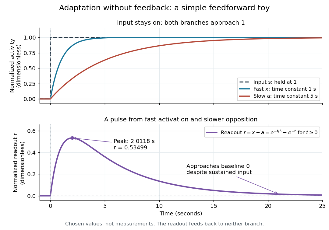
Find the pulse maximum by differentiating the exponential functions. With numerical time in seconds, the derivative isThe stationary condition is , so the natural logarithm givesBefore this time the derivative is positive; afterwards it is negative. Together with and , this proves that it is the unique pulse maximum. As another numerical check, at seconds , and : the slow branch is still catching up.
The subtraction is a mathematical readout, not a claim that an actual chemical concentration equals this difference for arbitrary inputs. Nonnegativity was established only for the specified upward step; other input histories can give a negative signed readout. Complete signaling adaptation here also relies on equal eventual branch gains: changing the readout to leaves for . This toy illustrates cancellation and different time constants; it does not establish molecular implementation or robustness to arbitrary parameter changes. Ma and colleagues' 2009 study separately analyzed biochemical mathematical models with negative feedback and incoherent feedforward loops, identifying additional conditions for signaling adaptation in those models. [ref]
https://cqb.pku.edu.cn/tanglab/pdf/78.pdf. Ma et al., Cell 138 (2009): adaptive architectures and their kinetic conditions
A historical connection to feedback control comes from Yi, Huang, Simon and Doyle's 2000 analysis of a bacterial chemotaxis model. They identified integral action in its regulation of receptor activity: accumulated deviations alter a slower adjustment, which in turn changes the measured activity. At a stationary state, an adjustment that integrates a nonzero error cannot remain constant, explaining how zero error can follow. Their conclusion depended on stated biochemical assumptions and stable behavior; it was not a claim that every biological cell uses that mechanism. A transient pulse alone, as the incoherent feedforward loop toy shows, cannot identify the underlying signaling feedback architecture. [ref]
https://groups.csail.mit.edu/mac/projects/amorphous/6.978/papers/doyle-PNAS-2000.pdf. Yi et al., Robust perfect adaptation in bacterial chemotaxis through integral feedback control, PNAS 97 (2000): Results and Discussion
Signaling feedback returns the effect of a downstream event to an earlier stage of signal transduction, closing a loop analogous to feedback control. Trace the causal arrows: if an earlier relay activates a later relay and the later relay changes the earlier relay's activity, the return path closes the loop. Negative feedback opposes the initiating change; positive feedback reinforces it. Signaling feedback is a possible property of signal transduction, not a requirement of every pathway.
For a schematic example, let relay activate relay . If inhibits , increased eventually produces an opposing influence: negative feedback. If activates , increased produces a reinforcing influence: positive feedback. These signs describe effects on activity, rather than the direction in which molecules travel. A closed loop containing two inhibitions can have positive feedback, because inhibiting an inhibitor reinforces the original change. The sign belongs to the whole loop.
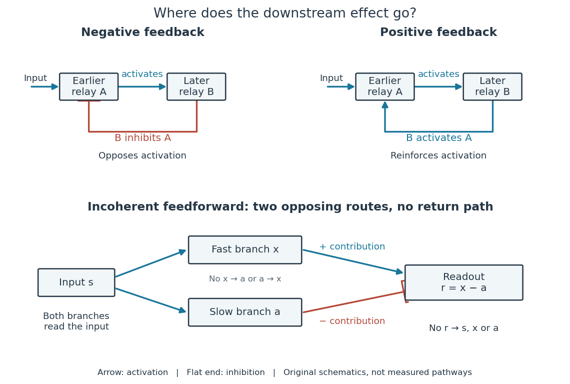
Negative feedback can restrain excessive activation and help preserve a usable range of responses. Positive feedback can support a decisive transition: Alberts and colleagues describe an enzyme whose product increases its own activity. Such reinforcement can contribute to switchlike behavior, but a positive feedback arrow alone does not prove bistability. A different structure, an incoherent feedforward loop, sends opposing influences forward from the same input; inhibition there is not a downstream return. [ref] [ref]
https://cqb.pku.edu.cn/tanglab/pdf/78.pdf. Ma et al., Defining Network Topologies that Can Achieve Biochemical Adaptation, Cell 138 (2009), pp. 760–773: definitions on p. 764
A worked mathematical model shows why negative feedback does not automatically produce complete signaling adaptation. Let be a fixed normalized input, a normalized response, a dimensionless feedback gain, and a time constant. Suppose response removal contributes and a return proportional to the response contributes . The ordinary differential equation isSetting the derivative to zero gives the equilibrium point . A displacement obeys , so its decaying exponential function establishes asymptotic stability. For a unit input switched on at , initial condition , and second,The negative feedback reduces the eventual response from to , but this response rises monotonically and never returns to its zero baseline. Attenuation and complete signaling adaptation are different properties. This deliberately simple mathematical model specifies no molecular pathway; integral action provides a contrasting way to remove a lasting offset in a stable feedback control system. [ref]
https://www.fbswiki.org/wiki/index.php/Feedback_Principles. Åström and Murray, Feedback Systems, Chapter 2: proportional and integral feedback
A hormone is a chemical messenger released by biological cells that regulates target biological cells bearing suitable receptors. In endocrine signaling, hormones travel to distant targets through the bloodstream. The extract-transfer experiment under second messenger isolates part of this signal transduction from intact biological cells. [ref]
https://openstax.org/books/biology-2e/pages/9-1-signaling-molecules-and-cellular-receptors. Clark, Douglas and Choi, Biology 2e, 9.1: hormonal signaling
Signal amplification is an increase in a specified downstream response relative to an initiating signal. In a molecular-count description, one activated component can generate or activate many downstream molecules. Repeated catalysis by an enzyme supplies a mechanism: the enzyme remains available for another chemical reaction. Successive stages can multiply the response. For a biological example, Cooper describes the epinephrine-to-glycogen phosphorylase pathway, where production of many cAMP molecules and repeated downstream protein phosphorylation provide opportunities for signal amplification. This is an example, not a claim that every signal transduction pathway has the same stages or gain. [ref]
Here is a counting toy extending the example under signal transduction. Suppose activated receptors each activate distinct relay proteins during a first interval. During a subsequent interval, each relay activates distinct target proteins. Assume enough inactive relays and targets, no shared targets, and no loss of activity during the count. ThenFor , this gives and : the target-to-receptor count ratio is . These are assumed integer counts, not measured rates or a universal physiological amplification factor. The intervals are sequential; the equations do not specify a time course.
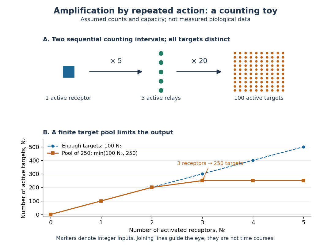
Availability limits the multiplication. As a second toy assumption, let there be only initially inactive target proteins shared by all branches, and suppose the branches can activate distinct targets until this pool is exhausted. ThenTwo activated receptors give active targets, whereas three give , not . At three activated receptors, the total count ratio is ; adding a fourth activates no additional targets. Thus total output per input and the increment caused by an extra input are different notions of gain. This finite-pool rule is an illustrative bound, not an enzyme kinetics law.
Signal amplification makes a small initiating signal capable of a larger response, but it does not supply the material or energy for downstream chemical reactions. In the second messenger transfer experiment, both stages still required added ATP and magnesium ions. Counts, changes in concentration, and changes in enzyme activity are different readouts; an amplification claim should name its input, output and observation interval. [ref]
https://doi.org/10.1016/S0021-9258(19)77422-5. Rall and Sutherland (1958), methods: production and assay of cAMP
A second messenger is a small intracellular molecule or ion that relays a received signal to target proteins. Its production, release, removal or binding changes its availability after signal reception. For a cell-surface receptor, distinguish the extracellular ligand, often called the first messenger, from the intracellular second messenger. An activated relay protein is not thereby a second messenger: the term identifies small chemical mediators, rather than every downstream component of signal transduction. [ref]
https://pubmed.ncbi.nlm.nih.gov/27481708/. Newton, Bootman and Scott, Second Messengers (2016): definition and classes
Two examples clarify what changes. A biological cell can make cAMP from ATP; alternatively, release of stored calcium ions can raise the free calcium concentration in its cytoplasm. The latter need not increase the total calcium content of the biological cell. Availability to target proteins, not merely the total amount present, carries the message. Removal and sequestration help terminate such signals. [ref]
https://www.ncbi.nlm.nih.gov/books/NBK10794/. Purves et al., Neuroscience, 2nd edition: second messengers and calcium storage
[ref]The experimental motivation is unusually tangible: can a hormone's effect be transferred to machinery that barely responds to the hormone itself? In Rall, Sutherland and Berthet's 1957 experiment, washed cat-liver particles were incubated with ATP and magnesium ions, with or without epinephrine and glucagon, two hormones. After five minutes at , the mixtures were heated in boiling water for three minutes, chilled, and separated to remove insoluble material. Small samples of the clarified extracts were transferred to a separate soluble dog-liver preparation, again supplied with ATP and magnesium ions. The readout was the change in glycogen phosphorylase activity over five minutes, not the amount of newly synthesized protein. [ref]
https://doi.org/10.1016/S0021-9258(18)65045-8. Rall, Sutherland and Berthet (1957), Figure 4 and pp. 470–471: preparation and transfer
The hormone-conditioned extract caused a larger increase in glycogen phosphorylase activity. Water, extract made without hormones, and hormones added directly to the soluble preparation produced smaller effects. These comparisons distinguish transferred activity from baseline activity, preparation effects and simple hormone carryover. [ref]
https://doi.org/10.1016/S0021-9258(18)65045-8. Rall, Sutherland and Berthet (1957), Figure 4: controls and observations
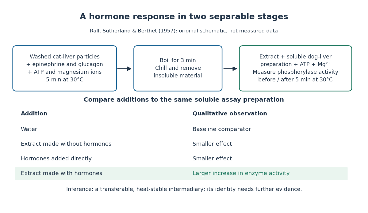
The inference is a transferable, heat-stable intermediary between the hormone-sensitive particles and the soluble machinery. This does not identify the intermediary merely from heat resistance, establish its direct target, or show that every hormone uses the same mechanism. Rall and Sutherland's 1958 paper reports the factor's identification as cAMP in accompanying chemical work, and follows its production from ATP. It also reports an important limit: washed heart and skeletal-muscle particles produced detectable cAMP with epinephrine under their test conditions, whereas brain particles produced similar amounts with and without it. Tissue and preparation matter. [ref]
https://doi.org/10.1016/S0021-9258(19)77422-5. Rall and Sutherland (1958), introduction and Table IV: cAMP identity and tissue-dependent responses
The useful and beautiful separation is between recognition and execution: an extracellular ligand can control intracellular enzymes through a chemically different intermediary. Making many second messenger molecules can support signal amplification, while different target proteins give the same mediator different consequences. A second messenger identifies a mode of relaying information; its presence alone does not specify the size or direction of the response. [ref]
https://pubmed.ncbi.nlm.nih.gov/27481708/. Newton, Bootman and Scott (2016): second messengers and their targets
A linear time-invariant system combines two properties. Linearity means that the output from a linear combination of inputs is the same linear combination of their outputs. Time invariance means that shifting an input by an integer delay shifts its output by exactly that delay. The operation has no preference for a particular time origin.
For discrete time, write the unit impulse as at and zero otherwise, a Kronecker delta. Its response is the impulse response. A finite input can be decomposed into shifted impulses, givingThe superposition principle supplies the sum and time invariance supplies the shifted copies of . Infinite sums need convergence assumptions; for a bounded input and an impulse response with absolute summability, the discrete convolution converges absolutely. For a physical system with stored initial energy, this construction describes the response with zero initial state; a separate free response accounts for nonzero initial conditions.
The gain is reuse. Measure or calculate one impulse response, and the convolution predicts the response to every allowed signal without solving a new dynamical problem each time. Alternatively, the frequency response predicts how each oscillatory component changes. [ref]
https://ocw.mit.edu/courses/res-6-007-signals-and-systems-spring-2011/0400ba59406d52d94c079d99928156ee_MITRES_6_007S11_lec04.pdf. Oppenheim, lecture 4: convolution from shifted impulses
.A linear filter obeys the superposition principle: filtering gives . Many familiar examples are also linear time-invariant systems, represented by an impulse response and convolution. Linearity alone does not imply time invariance: multiplying by the index is linear but changes its behavior when the same input is shifted.
The moving average is a finite impulse response example implemented by arithmetic; a band-pass filter can instead be built from a series RLC circuit. Their frequency responses explain which oscillations pass through. Choosing a filter means choosing how much amplitude, timing and detail may change, not simply removing every visible fluctuation.
A signal is a function or sequence representing a quantity that carries information. An electric potential difference measured over time can be written ; regularly recorded values give a discrete-time signal . The meaning includes the measured quantity, units, time reference and sampling interval. The same list of numbers sampled once per second or once per millisecond describes different physical frequencies.
An impurity that can supply an electron to the conduction band. A shallow donor has a localized occupied impurity level in a crystal near and below the conduction-band edge; thermal or other ionization releases its electron. The binding energy depends on the host dielectric response and effective mass.
An impurity that can accept an electron from the valence band, leaving a mobile hole. A shallow acceptor creates an impurity level in a crystal near and above the valence-band edge. Donor and acceptor levels are descriptions of appropriate dopants, not universal features of every impurity species.
A segment retained in the mature RNA after RNA splicing, or the corresponding segment of a gene. An exon need not encode a protein: the ribosomal RNA exons in the Tetrahymena ribozyme experiment are an example.
A segment represented in a precursor RNA that is removed by RNA splicing; the corresponding segment of a gene is also called an intron. An intron can interrupt ribosomal RNA as well as messenger RNA.
Sexual reproduction is reproduction involving fusion of gametes and a life cycle in which meiosis reduces the number of chromosome sets. Fertilization then combines parental contributions. Sexual reproduction can occur through self-fertilization in a hermaphrodite, so two separate individuals are not an essential part of its definition.
In a simple diploid example, a parent with two alleles at a genetic locus transmits one through each haploid gamete. Meiosis, genetic recombination and fertilization create new combinations of existing alleles; mutation supplies new sequence variants. Alternation of generations shows that a multicellular haploid phase can intervene between meiosis and production of gametes.
Budding produces a new individual from an outgrowth of its parent. In Saccharomyces cerevisiae, the daughter biological cell grows while attached to the mother and later separates; see the Burgess, Powers and Mell account cited there. Budding describes reproduction, not fermentation.
Asexual reproduction produces offspring without fusion of gametes. An operational species concept for such organisms needs evidence other than interbreeding.
An unpaired electron does not set a universal reaction rate. A stable radical can retain radical character during isolation and storage under specified conditions; a persistent radical survives long enough under specified conditions to be observed. These descriptions concern lifetime and handling, rather than immunity to every possible chemical reaction. DPPH is a practical counterexample to the claim that all free radicals react immediately.
Two mechanisms help explain persistence. Spreading electronic character over several chemical atoms, represented by chemical resonance, can lower the energy relative to a localized description. Bulky surrounding groups can impede approach to a reactive site and slow recombination. Lower energy and slower chemical kinetics are different advantages: neither alone guarantees a long lifetime. A primary computational study explicitly separates these effects, using electronic and geometric descriptors; it does not directly measure every predicted lifetime.[ref]
A quantitative metric for organic radical stability and persistence using thermodynamic and kinetic features by Shree Sowndarya S. V. and others. A quantitative metric for organic radical stability and persistence using thermodynamic and kinetic features, Shree Sowndarya S. V., Peter C. St. John and Robert S. Paton, 2021: Abstract and Introduction, thermodynamic stabilization versus kinetic persistence
A radical chain reaction regenerates a radical during propagation. Initiation supplies free radicals; propagation consumes one and produces another; termination removes chain-carrying free radicals. This explains why one initiating event can lead to many product-forming chemical reactions. The chain-growth polymerization article develops the corresponding growth of polymers.
A radical ion is both a radical and an ion. Removing one electron from neutral benzene can produce , a radical cation; adding one can produce , a radical anion. These formulae specify net electric charge and an unpaired electron, without claiming that both reside on one chemical atom.[ref]
Glossary of Terms Used in Physical Organic Chemistry (IUPAC Recommendations 1994): R entries by International Union of Pure and Applied Chemistry. Glossary of Terms Used in Physical Organic Chemistry, IUPAC Recommendations 1994: radical ion, benzene examples and dot/charge placement
The methyl radical is the neutral radical , with an unpaired electron. It carries the methane chlorination chain between its two propagation steps.
Molecular orbital theory describes the electronic arrangement of a molecule using molecular orbitals: one-electron spatial wavefunctions extending over the combined atomic nuclei. Filling bonding molecular orbitals can stabilize a chemical bond; filling antibonding molecular orbitals opposes that stabilization. A molecular orbital is a building block of a many-electron description, rather than the entire many-electron wavefunction. See Robert W. Field, MIT 5.61, lecture 24, pp. 1–4: molecular orbitals and the LCAO approximation.
First make the interference visible with an exactly normalized one-dimensional toy. Replace the three-dimensional atomic orbitals of the hydrogen atom by two Gaussian functions centred at , with dimensionless and :The normalized sum and difference are , following the same linear combination of atomic orbitals algebra. At , the orbital overlap is . At the midpoint, , givingBoth probability densities have total integral one: interference redistributes probability, rather than creating an extra electron. These are toy wavefunctions, not actual hydrogen atom orbitals or predictions of molecular hydrogen energies.
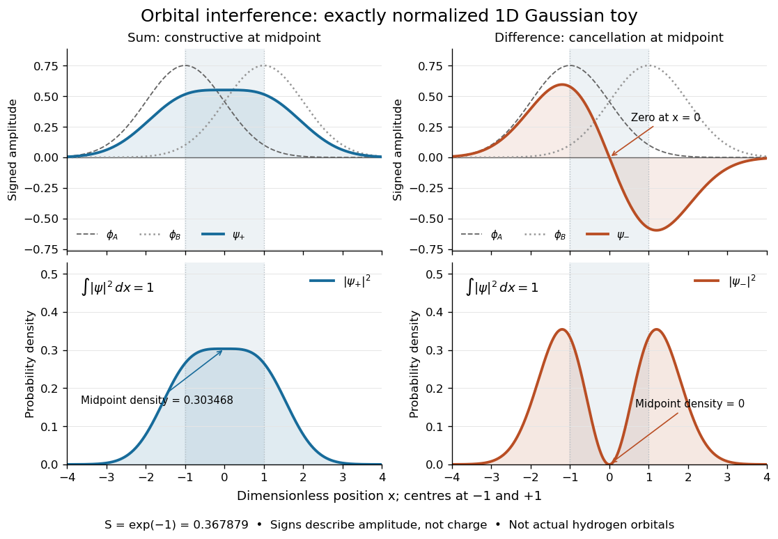
Normalized one-dimensional Gaussian function toy: signed probability amplitudes add or cancel before their squares give probability densities
. Centres at and give orbital overlap . The difference has a zero at the midpoint; its negative lobe does not carry positive electric charge. All density curves shown are normalized on the line, rather than in three-dimensional space. Details.Now fill the two -derived molecular orbitals in the minimal model. The lower bonding molecular orbital is labelled ; the upper antibonding molecular orbital is . The Pauli exclusion principle permits at most two electrons in each spatial molecular orbital, with opposite spin projections along a chosen axis. For the lowest electron configuration in this model, fill first. The subscripts and denote even and odd behaviour under inversion through the midpoint; the star marks an antibonding molecular orbital. See Flowers et al., Chemistry 2e, 8.4: occupancy and bond order and Field, MIT 5.61, lecture 25, pp. 1–3: bonding, antibonding, and symmetry labels.
With electrons in bonding molecular orbitals and in antibonding molecular orbitals, the model's bond order is . The three elementary counts are:
- Molecular hydrogen, : two electrons give and .
- The hydrogen molecular ion : one electron gives and .
- Two neutral helium chemical atoms, : four electrons give and in this minimal model.
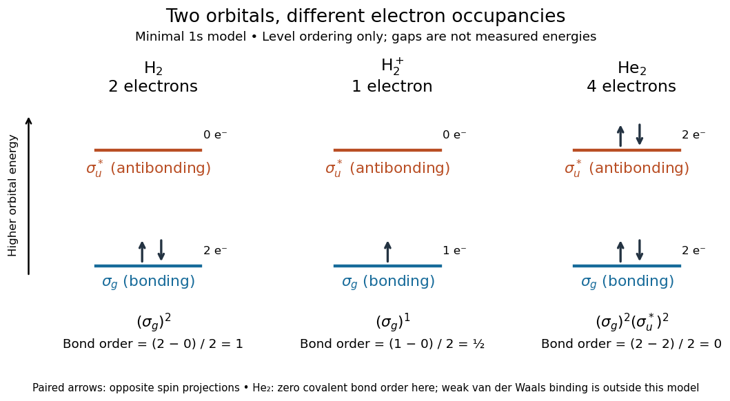
The zero bond order says this minimal model gives no net covalent bond for . It does not rule out every bound pair of helium chemical atoms: a very weak Van der Waals force can bind a neutral helium dimer, which has been observed experimentally. See Zeller et al., Imaging the He2 quantum halo state using a free electron laser, PNAS 113, 14651–14655 (2016), p. 14651: van der Waals binding and Luo et al., The weakest bond: Experimental observation of helium dimer, Journal of Chemical Physics 98, 3564–3567 (1993). The bond order count does not include that weak binding mechanism.
The useful surprise is that sharing alone does not determine a chemical bond: the relative quantum phase and the occupancy matter together. The same two shapes explain why adding an electron to a bonding molecular orbital increases the model's bond order, while adding one to an antibonding molecular orbital decreases it. Molecular orbital theory also accounts for the unpaired electrons and paramagnetism of molecular oxygen, which its all-paired Lewis structure misses. See Chemistry 2e, 8.4: the molecular orbital description of oxygen.
Pinned article: Introduction to the OurBigBook Project
Welcome to the OurBigBook Project! Our goal is to create the perfect publishing platform for STEM subjects, and get university-level students to write the best free STEM tutorials ever.
Everyone is welcome to create an account and play with the site: ourbigbook.com/go/register. We belive that students themselves can write amazing tutorials, but teachers are welcome too. You can write about anything you want, it doesn't have to be STEM or even educational. Silly test content is very welcome and you won't be penalized in any way. Just keep it legal!
Intro to OurBigBook
. Source. We have two killer features:
- topics: topics group articles by different users with the same title, e.g. here is the topic for the "Fundamental Theorem of Calculus" ourbigbook.com/go/topic/fundamental-theorem-of-calculusArticles of different users are sorted by upvote within each article page. This feature is a bit like:
- a Wikipedia where each user can have their own version of each article
- a Q&A website like Stack Overflow, where multiple people can give their views on a given topic, and the best ones are sorted by upvote. Except you don't need to wait for someone to ask first, and any topic goes, no matter how narrow or broad
This feature makes it possible for readers to find better explanations of any topic created by other writers. And it allows writers to create an explanation in a place that readers might actually find it.
Figure 1. Screenshot of the "Derivative" topic page. View it live at: ourbigbook.com/go/topic/derivativeVideo 2. OurBigBook Web topics demo. Source. - local editing: you can store all your personal knowledge base content locally in a plaintext markup format that can be edited locally and published either:This way you can be sure that even if OurBigBook.com were to go down one day (which we have no plans to do as it is quite cheap to host!), your content will still be perfectly readable as a static site.
- to OurBigBook.com to get awesome multi-user features like topics and likes
- as HTML files to a static website, which you can host yourself for free on many external providers like GitHub Pages, and remain in full control

Figure 2. You can publish local OurBigBook lightweight markup files to either OurBigBook.com or as a static website.
Figure 3. Visual Studio Code extension installation.
Figure 5. . You can also edit articles on the Web editor without installing anything locally. Video 3. Edit locally and publish demo. Source. This shows editing OurBigBook Markup and publishing it using the Visual Studio Code extension. 
- Infinitely deep tables of contents:




All our software is open source and hosted at: github.com/ourbigbook/ourbigbook
Further documentation can be found at: docs.ourbigbook.com
Feel free to reach our to us for any help or suggestions: docs.ourbigbook.com/#contact