For the force on a current loop in a bilinear magnetic field, the arrow gives current in the positive direction on the edge , and in the negative direction on the edge . Use . The edges on the coordinate axes contribute zero because the applied field vanishes there. The other two giveThus the force on the square itself, excluding the supply leads, isIt lies in the plane along the diagonal towards increasing and , at to either positive axis.
In the ideal semidiurnal tide model, successive high tides occur after the Earth–Moon relative angle advances by . Since the motions have the same sense, subtract their angular speeds:The lunar orbital period is sidereal, so the consistent terrestrial rotation period is . With , this gives about 12 h 25 min. The sidereal terrestrial period is distinct from the 24-hour solar day.[ref]
Earth Fact Sheet by National Aeronautics and Space Administration. Orbital parameters, sidereal rotation period 23.9345 h and length of day 24 h
If the Earth's rotation is approximated as one revolution in 24 hours, the same calculation instead gives 12 h 27 min. That small difference is the day convention, not a change of sign in the relative angular speed. Actual coastal tide times also depend on ocean dynamics and the solar tide.
For the uniform magnetic field in an off-axis cylindrical cavity, let point from the conductor's axis to the hole's axis and let the current flow in . Its uniform current density in the metal isSuperpose a complete cylinder carrying and a cylinder occupying the hole carrying . Inside a uniformly filled cylinder, Ampère's law gives . For any point in the cavity,There is no remaining position dependence, so the field is uniform. Its magnitude is , perpendicular to the axis-offset vector in the cross-sectional plane. Reversing the current reverses the field.
Use the rotating reference frame equilibrium model, in which the centrifugal potential energy of a particle of mass is . The Boltzmann distribution then givesDefine the concentration ratio as . At the axis,Thus the axis favours the lighter species. The expression assumes a dilute classical mixture at one temperature, equilibrium in the rotating reference frame, and sampling sufficiently close to .
Define , where counts particles in the level. Then , soThe binomial entropy of independent two-level particles follows from counting which of the independently labelled particles occupy each nondegenerate level. This is the usual distinguishable, or localized, two-level model; occupation constraints of a degenerate quantum gas would require different counting.
For large occupations, Stirling's approximation with givesAllowed runs from to in steps of two. Entropy is largest near equal populations and is zero when all particles occupy one level; use at the endpoints.
In vacuum, displacement current contributes the additional term :Taking the divergence and using Gauss law gives , the local conservation of charge. Without displacement current the curl equation would incorrectly require a divergence-free current even during charge accumulation.
For a charging capacitor, a surface cutting the wire carries conduction current while a surface passing through the gap carries changing electric flux. The displacement current term makes the circulation independent of the spanning surface. It is not transport of free charge across the vacuum gap. In matter the macroscopic equation is , with electric polarization included in . Together with Faraday's law of induction, the vacuum equations give electromagnetic waves of speed .
An applied electric field displaces bound charges or reorients permanent dipoles, producing electric polarization , the dipole moment per unit volume. It gives bound charges and . Definefor a linear isotropic dielectric. Then separates free charge from the bound-charge response. Electronic, ionic and orientational electric polarization respond on different timescales; real permittivity is frequency dependent, and its dissipative part describes dielectric loss.
A uniform dielectric filling a parallel-plate capacitor raises its capacitance to . At fixed charge this reduces field energy ; at fixed voltage the stored energy increases because the voltage source supplies charge and energy. Insulation and energy storage are useful applications, limited by loss and dielectric breakdown. Static interface conditions are continuous tangential and a jump in normal equal to free surface charge.
A current in one circuit links magnetic flux through another. It produces magnetic flux linkage through another. With fixed geometry and a linear reciprocal medium, choose consistent winding orientations and writeThe shared coefficient is mutual inductance; reversal of one winding reverses its sign. Faraday's law of induction gives the mutual induced emf for fixed . The minus sign expresses Lenz's law.
The magnetic energy isNonnegative energy for every current pair requires , motivating the coupling coefficient . Transformers use strong common flux to exchange energy between circuits; leakage flux reduces coupling. A shared core increases linkage, but saturation, hysteresis and eddy-current losses limit the linear description. A moving geometry also contributes to the mutual emf.
Find the potential from and . One must specify boundary data: a potential on each Dirichlet boundary, a normal displacement on each Neumann boundary, or an appropriate mixture. Conductors are equipotentials; at dielectric interfaces is continuous and the normal displacement jumps by the specified free surface charge. With no singular dipole sheet, tangential electric field is continuous.
To establish uniqueness of Poisson equation, subtract two solutions with the same charge and boundary data, writing their difference as . Integration by parts givessince . The right side vanishes for identical Dirichlet data, identical Neumann data, or their usual mixed combination. Interface terms cancel under the homogeneous difference conditions. With positive permittivity, : the field is unique, and the potential is unique if any suitable reference potential is fixed. For a pure Neumann problem an additive constant remains, and the prescribed outward displacement flux must equal the enclosed free charge. This theorem justifies image-charge solutions once their boundary data have been checked.
Magnetization is magnetic dipole moment per unit volume. In SI units,in a linear isotropic response. The internal field matters: for a uniformly magnetized ellipsoid it is . Sample shape therefore affects an apparent magnetic susceptibility.
Diamagnetism opposes the applied field, giving small negative magnetic susceptibility from the induced orbital response. It is often only weakly temperature dependent. Paramagnetism aligns pre-existing moments and gives positive magnetic susceptibility; independent localized moments obey approximately in weak fields before saturating. Pauli paramagnetism of conduction electrons is a different, weakly temperature-dependent mechanism.
Ferromagnetism involves collective exchange-driven alignment and spontaneous magnetization below the Curie temperature. A specimen can nevertheless have nearly zero total moment because magnetic domains point in different directions. Field-driven domain-wall motion and rotation change the net magnetization. Antiferromagnets have compensating ordered sublattices below a Néel temperature; ferrimagnets have oppositely ordered but unequal sublattice moments and retain a net moment. Ferrites are useful examples of electrically resistive ferrimagnetic core materials.
Ferromagnetic response is nonlinear and history dependent. A hysteresis loop displays remanent magnetization, magnetic coercivity and saturation. A single constant magnetic permeability cannot describe the entire loop: differential magnetic permeability describes its local slope. The quasistatic energy loss per unit volume and cycle is the loop area . Soft magnetic materials have low magnetic coercivity and usually high useful magnetic permeability; hard magnetic materials retain magnetization and suit permanent magnets.
An electromagnet normally uses a soft, high-permeability core to guide flux generated by a coil. For a uniform-section core with length and air gap , neglecting leakage and fringing,An air gap can dominate the magnetic reluctance even when the core magnetic permeability is large. Core saturation limits the improvement with current, while winding resistance causes heating. For alternating operation, laminations suppress eddy-current loops in metallic cores; high-resistivity ferrites also reduce those losses. Low hysteresis loss is important in repeatedly cycled cores, whereas high magnetic coercivity is valuable in a permanent magnet. Useful design therefore depends on the full magnetic response, electrical losses and operating frequency, rather than the largest quoted magnetic permeability alone.
Generalized coordinates incorporate holonomic constraints without solving separately for every constraint force. For conservative mechanics use . The principle of stationary action makes the action stationary for variations vanishing at the endpoints. Integration by parts givesThe canonical momentum is . A cyclic coordinate gives conserved ; absent explicit time dependence, is conserved. These are symmetry–conservation relationships, not assumptions that all momenta are constant. Nonconservative generalized forces enter the right side.
For example, a pendulum has , giving . The method extends directly to coupled coordinates and velocity-dependent interactions when the correct Lagrangian is used; with a position-only potential is not the most general form.
Viscosity transfers momentum between adjacent fluid layers. A Newtonian fluid has shear stress proportional to strain rate: for simple shear, . Thus parallel plates of area , separation and relative speed require force magnitude in a steady linear profile.
For an incompressible isotropic Newtonian fluid,for constant viscosity. With strain-rate tensor , the viscous dissipation rate per unit volume is . Kinematic viscosity is the momentum diffusivity: a disturbance spreads over distance of order .
The Reynolds number compares inertial and viscous forces. Small Reynolds number supports a creeping-flow approximation, while large values permit thin viscous boundary layers and possible turbulence. It does not mean molecular viscosity has disappeared. Gas viscosity results from molecular momentum transport; a liquid's microscopic transport depends strongly on intermolecular interactions. Non-Newtonian materials require a more general constitutive law.
For an attractive inverse-square potential, let the reduced mass be , potential , and nonzero orbital angular momentum . Conservation of angular momentum makes the orbit planar. The orbit equation isPositive relative energy gives and an unbound hyperbolic Kepler orbit, arriving from and returning to infinity. Its asymptotes satisfy . At infinity and for impact parameter , so the deflection angle isThis describes gravitational encounters in the Newtonian two-body approximation. The body speeds up near periapsis while total energy remains positive. It is distinct from an elliptic bound orbit and from the zero-energy parabolic limit; repulsive Coulomb scattering also gives hyperbolae but uses a different orientation of the force and orbit.
For a homogeneous isotropic solid with small displacement , linear elasticity gives . Momentum balance becomesA plane wave with displacement parallel to its wavevector is longitudinal, whereas perpendicular displacement is transverse. Writing for the bulk modulus and for the shear modulus, their bulk speeds areThere are two independent transverse polarizations. The bulk modulus supplies resistance to compression; shear rigidity supplies transverse restoring stress. An ordinary fluid has no static shear rigidity and cannot sustain these propagating bulk shear waves. A thin rod with freely contracting sides instead has longitudinal speed , because its lateral boundary conditions differ from a bulk plane wave. Reflection, refraction and mode conversion occur at interfaces; a free surface also supports Rayleigh waves.
For torque-free rotation, angular momentum is fixed in inertial space, but angular velocity need not point along it. In principal body axes,and cyclic permutations. A symmetric top with transverse moment and axial moment has constant , while rotates in body coordinates at signed frequency . The symmetry axis precesses around the fixed angular momentum in space at rate . These body-frame and space-frame rates describe different motions and need not coincide.
Poinsot construction expresses the same torque-free motion geometrically. The energy ellipsoid is fixed in the body. Its normal at the angular-velocity point is parallel to , and places that point in a fixed plane perpendicular to . The ellipsoid rolls on this invariable plane without slipping: the instantaneous velocity of its contact point is proportional to . The contact curve is the polhode on the body ellipsoid and the herpolhode on the plane.[ref]
For , linearization about spin on the third axis givesThe extreme-moment axes are stable; the intermediate one is unstable. The major-axis relaxation theorem adds weak internal dissipation while retaining negligible external torque. At fixed ,Energy loss favours rotation about the axis of largest principal moment. Here “major axis” means maximum inertia, not necessarily the body's longest geometric direction. A perfectly rigid torque-free body does not dissipatively settle; its energy is conserved. Distinguishing stability from relaxation also explains why minimum-inertia rotation can be stable in the ideal rigid model.
Forced precession occurs when an external torque changes , with . For steady precession, . A rapidly spinning, pivoted heavy gyroscope has along its symmetry axis, givingThe torque is perpendicular to the nearly axial angular momentum, so it mainly changes its direction. For a steady inclined symmetric top, the more complete condition isIt exhibits slow and fast precession branches when real solutions exist. A generic release excites nutation as well: inclination oscillates instead of staying fixed. Axis constraints and bearing forces must be included when specifying which angular momentum and pivot are being used.
For speed distribution normalized to one and isotropic directions, the incident number flux isThe positive normal velocity weights the population reaching the wall. Consequently its mean translational energy isThe bulk value would omit the arrival weighting.
For the two vessels, let , with subscripts h and c for hot and cold. Equal opposing effusion rates give . Number conservation in equal, fixed volumes adds . HenceBoth final pressures must be determined; holding the cold temperature fixed does not hold its particle number fixed.
For aperture area , the common one-way flux is . The translational heat transfer from hot to cold is thereforeThis is the total heat transfer for a monatomic gas with no active internal modes, neglecting radiation and conduction through vessel walls. For a molecular gas, add for its internal energy per molecule. The maintained unequal temperatures describe a stationary nonequilibrium state even though the net particle current is zero.
A thermodynamic potential packages the equilibrium state in variables suited to the imposed constraints. For a simple fluid, has differential . Legendre transforms give , and , with natural variables of a thermodynamic potential , and respectively. At fixed particle number, Helmholtz free energy is minimized at fixed ; Gibbs free energy at fixed .
A flow vessel is an open control volume, even if its walls are enclosed. For each inlet, pressure forces carry flow work in addition to internal energy. The steady first-law balance isWith no heat exchange, shaft work, or significant kinetic and gravitational energy differences, the enthalpy fluxes are equal. Mass flow must also balance. This equality concerns mass-flow-weighted specific enthalpies, not an unweighted sum over pipes.
Using for the printed specific enthalpy, the formal outlet mass balance givesFor fixed outlet enthalpies the greatest yield occurs at the smallest inlet enthalpy. Among the tabulated pressures this is 30 atm. Approximating the atmospheric-pressure gas enthalpy by the tabulated zero-pressure limiting value givesThis uses a low-pressure approximation: atm is not literally the zero-pressure table entry. Linear interpolation to 1 atm would instead give and . The sparse table does not determine an exact continuous optimum between entries.
TODO: a physically consistent liquid fraction requires corrected outlet conditions and their corresponding gas and liquid enthalpies. The printed claim that the outlet contains liquid at 14 K and atmospheric pressure is inconsistent with helium's critical temperature near 5.2 K and normal boiling point near 4.224 K. The formal calculation above therefore is not a physically realizable 14 K liquefaction yield; the supplied states must not be silently replaced.[ref]
A heat pump delivers : electrical work moves heat from a source as well as contributing energy itself. Its heating coefficient of performance can therefore exceed one, whereas direct resistance heating supplies at most its electrical input as useful room heat. For an ideal reversible pump,with absolute temperatures and . This is an ideal limit; actual costs also depend on compressor performance and tariffs.
For the annual ground-temperature wave, model the soil as a homogeneous semi-infinite conductor, with depth positive downward and a prescribed surface temperature. Here is thermal conductivity and is heat capacity per unit volume, so the thermal diffusivity is . Conservation of energy gives . After transients decay, put . Substitution gives ; the solution bounded at depth uses . Matching the surface then givesThis approximation identifies the ground surface with air temperature and neglects the pump's perturbation of the ground, as required by the model. The attenuation and phase delay arise from heat diffusion, not propagation at one fixed wave speed.
The graph below covers a full annual cycle. At , the amplitude is K and the minimum lags January by a quarter-year. At , the amplitude is only K and the minimum lags by half a year: the ground is slightly warmer than its annual mean in January.
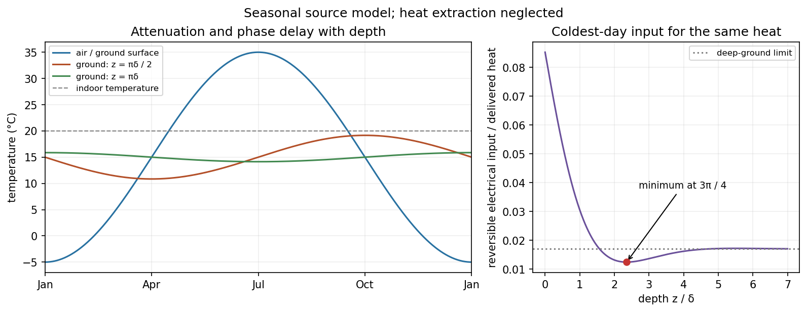
Annual air and ground temperatures, with attenuation and depth-dependent phase delay
. Details. 
The seasonal source depth for a reversible heat pump has a subtle limit: a deep source approaches and avoids severe winter cooling, but infinite depth is not the thermal optimum of this single-frequency model. In January, with , maximize . The first and largest maximum is at , where , giving and . It is also the optimum of the ideal annually integrated heating work: the heating load is even about January, so its weighted sine term integrates to zero and the depth dependence is again proportional to . Installation cost, finite tube spacing, heat extraction, weather and real pump performance alter this result. The supplied model therefore supports a finite seasonal thermal optimum, while not fixing a practical burial depth in metres.
The coldest day has outside temperature , so the indoor–outdoor temperature difference is 25 K. If is the building's heat-loss coefficient, the required heating rate is . For direct electrical heating,This sets the reference electrical cost for the same delivered heat and tariff.
For the ideal reversible comparison, K and the coldest air source is K. ThusA real air-source pump uses more work than this reversible lower bound, and its low-temperature performance is not specified.
A source much deeper than the annual penetration depth has K. ThereforeThe ideal coldest-day electrical-input ratios are direct : air-source : deep-ground = 1 : 0.0853 : 0.0171. The deep source needs one fifth of the ideal air-source work. These ratios compare equal useful heating, and do not include excavation, circulation losses or an assumed real compressor efficiency.
Phase equilibrium minimizes Gibbs free energy at specified temperature, pressure and composition. Coexisting phases have equal temperature, pressure and chemical potential. For a pure substance, a first-order transition has continuous equilibrium Gibbs free energy but a jump in its first derivatives, such as entropy or volume; the latent heat is . Continuous transitions lack that latent heat and can instead have singular or discontinuous higher responses.
The van der Waals molar equationcombines an excluded-volume correction with attractive interactions. Its inflection conditions giveBelow , the oscillatory isotherm contains a mechanically unstable segment with . Equilibrium instead replaces the loop by a constant-pressure coexistence line. Equality of chemical potentials gives the Maxwell construction,On isothermal compression the gas reaches saturation, then converts progressively into liquid at fixed pressure. The mean molar volume obeys , where is the gas fraction. Metastable superheated or supercooled states can persist when nucleation is delayed; they are not the global equilibrium selected by this construction.
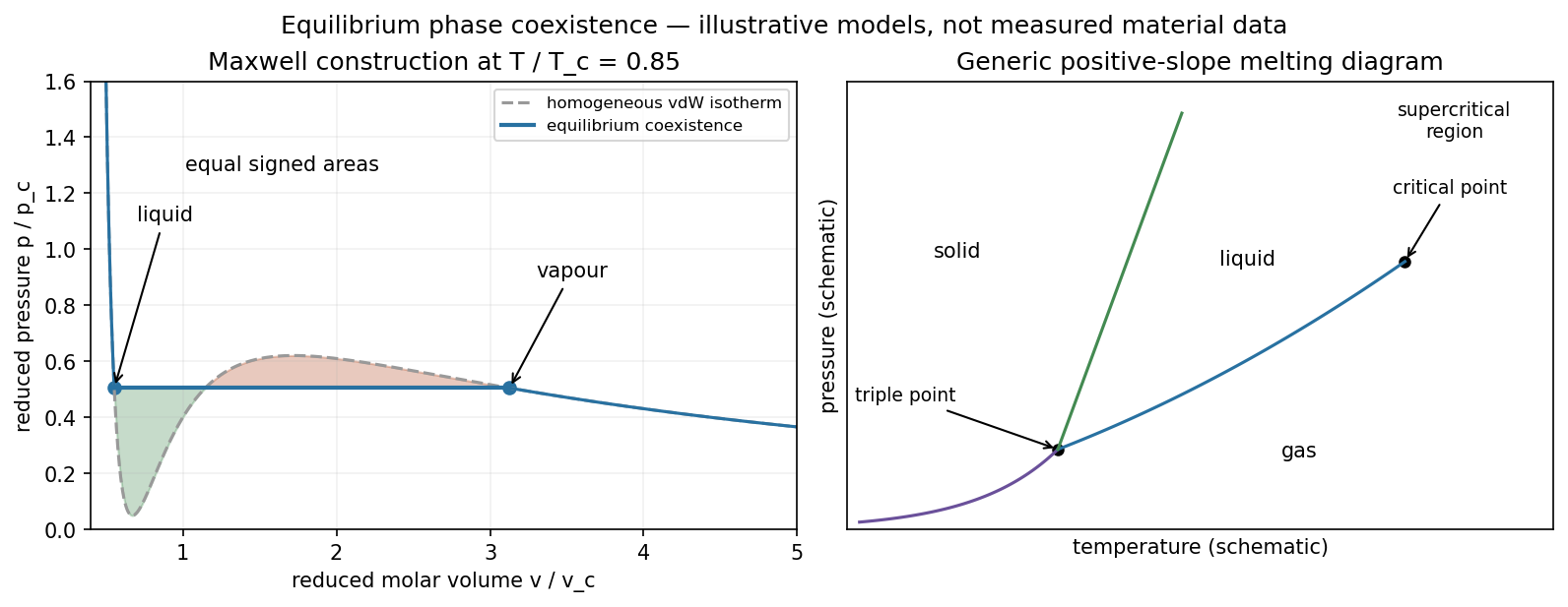
Illustrative reduced van der Waals coexistence and a generic pure-substance phase diagram
. Details. 
A pressure–temperature phase diagram contains coexistence curves separating solid, liquid and gas. Three phases meet at a triple point; the liquid–gas coexistence curve ends at a thermodynamic critical point, above which liquid and gas can be connected without crossing a first-order phase boundary. A generic solid–liquid line continues beyond the liquid–gas critical temperature. For one component the Gibbs phase rule is , so a three-phase equilibrium fixes both temperature and pressure.
Along a two-phase coexistence curve, for each phase givesThis is the Clapeyron equation, valid with consistent molar or specific quantities. For vaporization, neglecting the liquid volume and treating the vapour as ideal gives , hence . With approximately constant molar latent heat,This Clausius–Clapeyron approximation explains the rapid rise of vapour pressure with temperature. It fails close to the thermodynamic critical point, where phase volumes converge, and is not a universal expression for melting. The sign of a melting-line slope depends on its volume change; water's denser liquid gives a familiar negative slope.
Articles by others on the same topic
There are currently no matching articles.