Topics (384k) Articles (398k) Users (410) Discussions (242) Comments (383) Files (13k) New article

The Portable Operating System Interface standards specify interfaces and observable behaviour for portable programs, including file descriptors, hard links and unlinking an open file. Their requirements do not prescribe one on-storage inode layout. The worked examples below use POSIX Unix semantics for ordinary files. [ref]
https://pubs.opengroup.org/onlinepubs/9799919799/basedefs/V1_chap03.html. The Open Group, POSIX.1-2024, definitions of files, directories and file descriptors
// Target: computer-science.bigb
A nuclear reaction transforms one or more atomic nuclei through interactions with particles or other nuclei. Total energy, momentum, electric charge and nucleon number constrain ordinary low-energy reaction bookkeeping. Nuclear fusion, alpha capture, neutron capture and photodisintegration are important examples in stellar nucleosynthesis. Weak processes can also change the proton-to-neutron ratio.
Nucleosynthesis is the production of atomic nuclei through nuclear reactions. It includes Big Bang nucleosynthesis, stellar nucleosynthesis and production in explosive or compact-remnant environments. Making nuclei and delivering them to the interstellar medium are separate steps in chemical enrichment.
Capture of a neutron increases mass number without immediately changing atomic number. It avoids the charged-particle Coulomb barrier. Subsequent beta-minus decay can increase atomic number. Whether capture is slow or fast compared with relevant beta decays distinguishes the slow neutron-capture process from the rapid neutron-capture process.
At sufficiently high temperature and density, forward and inverse nuclear reactions can balance so that abundances are determined by thermodynamic conditions, nuclear binding and conserved quantities. Silicon burning approaches such an equilibrium among iron-group nuclei. Weak reactions can separately change the electron fraction, so the favored mixture need not be pure iron.
A nucleus bound in a solid can emit or absorb a photon without exciting lattice vibrations, transferring momentum to the solid as a whole. The resulting recoil energy is negligible compared with the isolated-nucleus recoil, making very narrow resonant emission and absorption lines observable. The Pound-Rebka experiment uses this effect to resolve the small frequency shift from gravitational redshift.
The striking feature is the combination of a large photon energy and a tiny natural linewidth: an atomic nucleus can act as an extraordinarily selective energy filter. The Mössbauer effect supplies a narrow shared emission line and absorption line even when nuclear recoil would separate the corresponding free-nucleus lines. A slow mechanical motion can then tune their overlap through the Doppler effect. The Pound-Rebka experiment is an application to general relativity; the discovery experiment below concerns the recoil-free process itself.
Mathematical and computational models connect neural mechanisms, measured responses and proposed information-processing functions. Their predictions require comparison with experiments; matching observations does not uniquely identify the biological mechanism.
Patch clamp connects an electrode to a small area of cell membrane through a solution-filled patch pipette. A gigaohm seal around the rim makes tiny electric currents through ion channels distinguishable from seal leak current. The beautiful change of scale is from a population's average response to individual opening and closing events in single-channel recording.
Separate two questions. The configuration determines which cell membrane is accessible: an intact patch in cell-attached recording, an excised inside-out patch or outside-out patch, or intracellular access in whole-cell recording. The recording mode determines what is commanded and what is observed: voltage clamp commands an electric potential difference and measures electric current; current clamp commands electric current and measures membrane potential. Whole-cell recording supports both modes. A patch can contain several ion channels; a small recording area does not establish that only one is present.
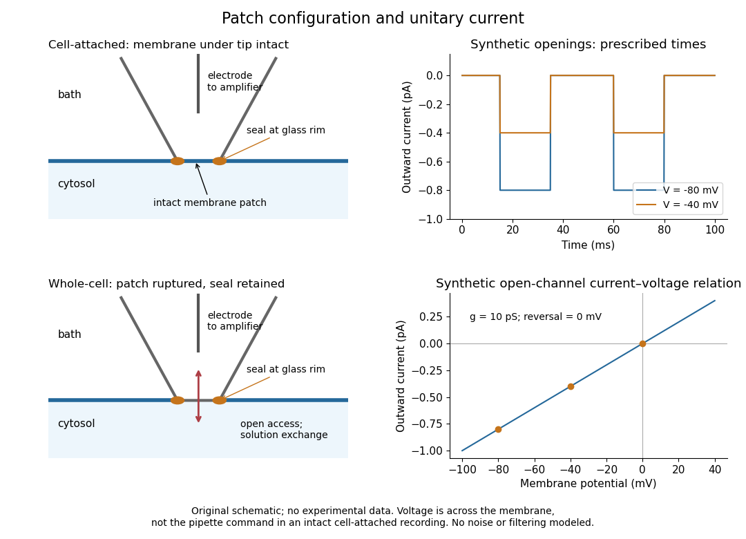
Patch clamp configurations and synthetic single-channel recording
. Original schematic of cell-attached recording and whole-cell recording, with synthetic electric current traces and a single-channel current-voltage relation. The prescribed opening times are identical at and solely to compare amplitudes. These are not experimental data or a model of opening probability. Membrane potential means the actual voltage across the patch, not automatically the pipette command. Details.The 1976 article Single-channel currents recorded from membrane of denervated frog muscle fibres describes an extracellular fire-polished pipette with a – opening and – electrical resistance. It contained saline and a channel-activating compound. Two separate intracellular electrodes supplied local voltage clamp of the muscle fibre; the patch amplifier measured local electric current. Cooling to – and hyperpolarization helped resolve elementary events. Figure 2 shows step-like pulses with a filter at and . Discrete amplitudes and overlapping events supported individual ion channel openings rather than a smoothly varying population response. This was neither whole-cell recording through the patch pipette nor current clamp. The specialized conditions improved visibility but limit generalization to warmer preparations; filtering can conceal brief openings.[ref]
Single-channel currents recorded from membrane of denervated frog muscle fibres by Erwin Neher and others. p. 800, Figures 1–2 and accompanying experimental conditions
For a new single-channel recording experiment, useful controls include a matched recording without the activating compound, controlled membrane potential, repeated seal tests, and an explicitly stated filter frequency response. These are proposed controls, not claims that every one was performed in that 1976 figure. Changing membrane potential tests the single-channel current-voltage relation; changing the recording filter tests whether a short pulse's apparent amplitude is an instrument artifact. A flat baseline establishes neither an absence of ion channels nor an absence of very brief events.
The retina is the layered neural and supporting tissue at the inner posterior eye. Photoreceptors convert light into signals processed by retinal circuits, and retinal ganglion cells supply output through the optic nerve. Spatial sampling and processing begin before signals reach the brain.
A neuron is a specialized biological cell that receives, integrates and transmits signals. Its shape separates places where inputs arrive from places where outputs reach other biological cells: this functional asymmetry is neuronal polarity. Understanding a neuron therefore means connecting its anatomy to changes in membrane potential, rather than treating it as a wire that merely forwards every input.
In a common multipolar neuron, branching dendrites receive inputs at synapses; the soma contains the cell nucleus and most major organelles; the axon carries signals to distant or nearby targets; and axon terminals form output contacts. All these regions belong to one biological cell enclosed by a continuous cell membrane. An axon can branch, allowing one neuron to influence several receiving biological cells.[ref]
12.2 Nervous Tissue. §12.2, Parts of a Neuron: nucleus, organelles, processes, branching axon, initial segment and terminals
At an input chemical synapse, a neurotransmitter acts on a receptor, changing an electric current directly or through signal transduction.[ref]
3.1 Synapses. §3.1, opening paragraphs: ionotropic and metabotropic receptors and postsynaptic currents
A resulting synaptic potential contributes to synaptic integration in the dendrites and soma. In many spiking neurons, sufficiently strong depolarization recruits voltage-gated ion channels in the axon initial segment, initiating an action potential that propagates along the axon. At an output chemical synapse, calcium entry through voltage-gated ion channels promotes synaptic vesicle exocytosis, releasing neurotransmitter. An action potential is thus regenerated electrically along a cell membrane; it is not a packet of neurotransmitter travelling from the dendrites to the axon terminals.[ref]Neuroscience, 2nd edition edited by D. Purves and others. Chemical Synapses, Figure 5.3: voltage-gated calcium entry and synaptic vesicle exocytosis
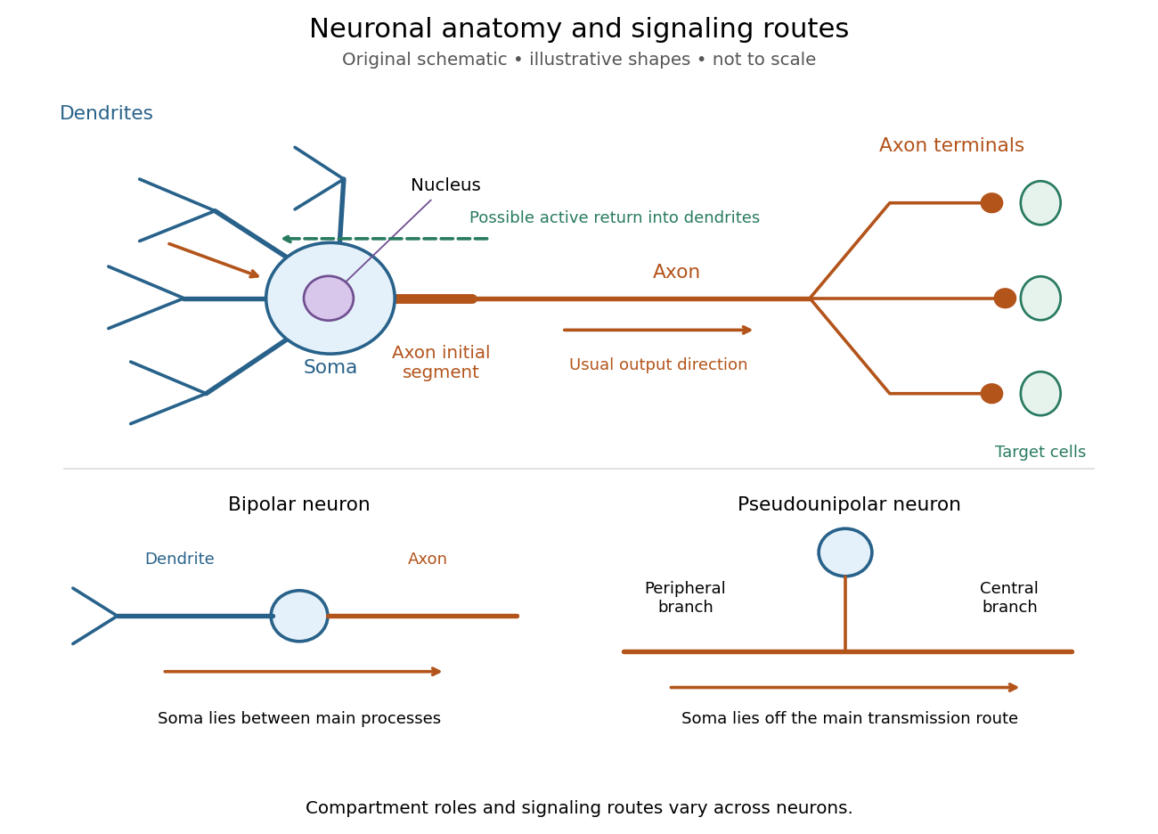
The compartments are specializations, not exclusive jobs. Inputs can contact the soma or axon as well as dendrites; dendrites can support active voltage-gated ion channels. Paired recordings from a pyramidal neuron's soma and dendrite or axon established that an action potential can begin in the axon and propagate back into the dendrites. The usual output direction therefore does not make every electrical signal strictly one-way.[ref] An electrical synapse, which directly couples cytoplasms through gap junctions, also differs from the sending-and-receiving arrangement of a chemical synapse.[ref]
Nor does every neuron have the upper diagram's shape. A bipolar neuron has two main processes, one dendrite and one axon; a multipolar neuron has several dendrites; and a pseudounipolar neuron has a single process from the soma that divides into peripheral and central branches. In the last arrangement, sensory signals can travel past the soma rather than obligatorily through it. These shape categories do not specify every neuron's receptor, connectivity or firing behavior.[ref]
12.2 Nervous Tissue. §12.2, Types of Neurons and Figure 12.9: multipolar, bipolar and human pseudo-unipolar cells; sensory projection past the cell body
Some neurons in the retina communicate through graded changes in membrane potential without generating action potentials.[ref]Why timing changes the computation. Synaptic integration can combine inputs at different locations, called spatial summation, and inputs arriving at different times, called temporal summation. A minimal example uses the leaky integrate-and-fire model with the illustrative parameters already given there: resting and reset membrane potential , firing threshold , electrical resistance , capacitance , time constant and neuronal refractory period . These are chosen model values, not measured properties of a particular neuron. Before firing, a constant inward electric current starting from rest givesThe exponential function expresses the competition between charging the cell membrane's capacitance and leakage through its electrical resistance.[ref]
Two inputs, each lasting , produce different outputs depending on their timing. Either input alone reaches only . Applied together, they give and reach threshold after , producing one action potential event during the pulse. If instead the second input begins after the first ends, the earlier depolarization has partly decayed: the second pulse peaks at approximately and neither pulse produces an action potential. The two-input protocols deliver the same total electric charge, , yet only the coincident protocol fires. Counting total input alone misses this timing dependence.
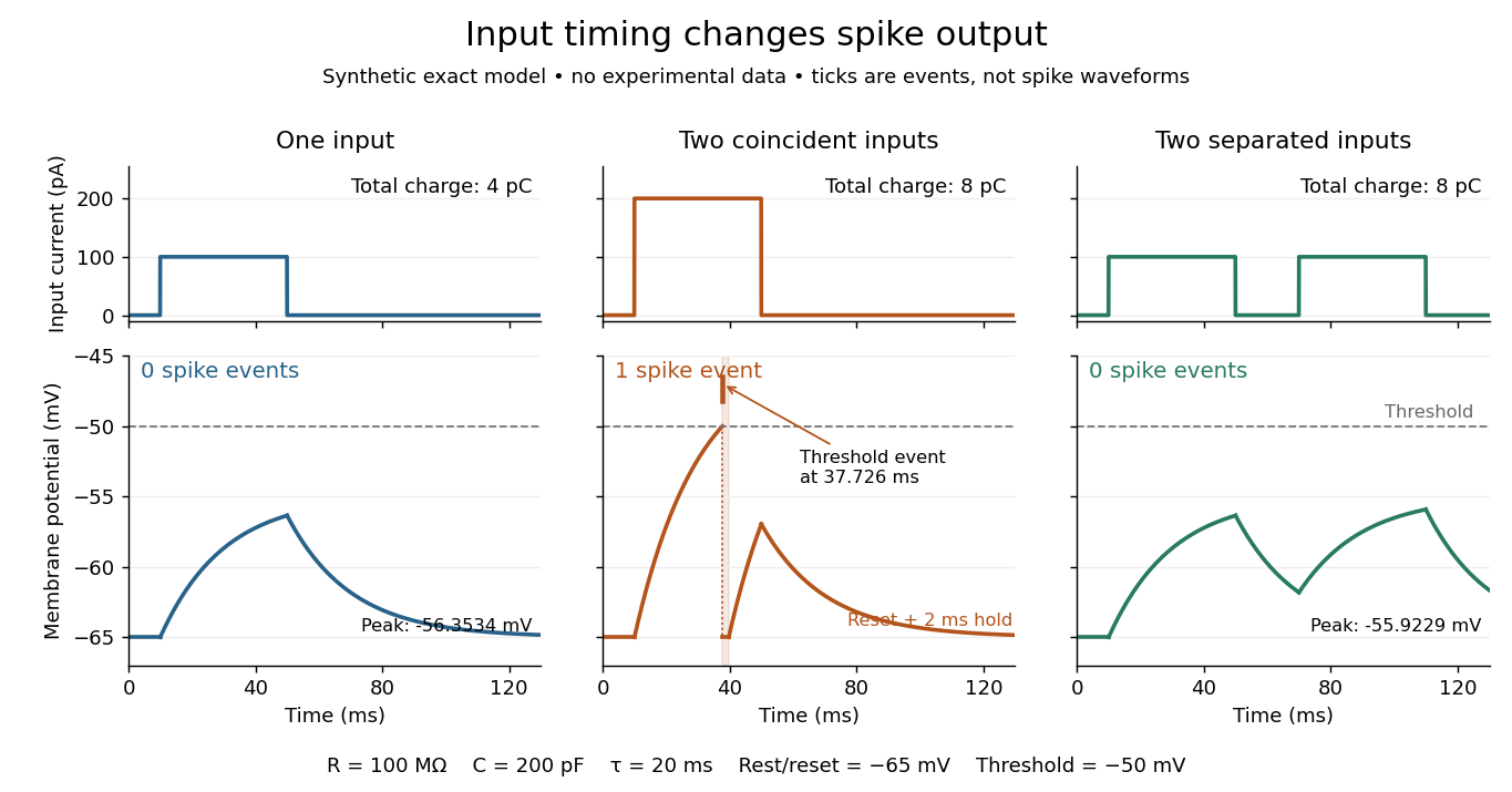
The same total input can yield different neuronal outputs
. Synthetic exact leaky integrate-and-fire model responses, not empirical recordings. A single pulse is below threshold; two coincident pulses produce one action potential event, shown as a tick rather than a biological waveform; two separated pulses deliver the same total electric charge as the coincident pair but produce no events. The lower traces show membrane potential, its reset and the brief neuronal refractory period. All inputs are prescribed electric currents in a single compartment, without a modeled synaptic conductance or spatial dendrite. Details.This example makes a neuron a detector of sufficiently clustered input, not a perfect logical gate: different parameters change the result. Actual dendrites introduce location-dependent filtering and active responses, and an inhibitory postsynaptic potential or shunting inhibition can change whether another input succeeds. The single-compartment leaky integrate-and-fire model omits these mechanisms.[ref]
1.4 Limitations of the Leaky Integrate-and-Fire Model. §1.4.2 and §1.4.4: shunting inhibition, spatial structure and active dendritic responses
Across connected neurons, branching axons distribute outputs while converging synapses combine inputs; spike trains can support temporal coding and rate coding, and synaptic plasticity changes the influence of an input. Connectivity and cellular dynamics together determine the computation.[ref][ref]Testing the connection between structure and function. Whole-cell recording connects anatomy to a measured membrane potential. In a published mouse protocol, a two-photon microscope guides solution-filled glass pipettes to neurons; an amplifier and bath reference electrode complete the electrical recording apparatus. A high-resistance seal forms against the cell membrane, then brief suction opens the membrane patch beneath the tip. In current clamp, the amplifier supplies a chosen electric current and records the resulting membrane potential, unlike voltage clamp, which controls voltage and measures electric current. The investigators used current steps of several amplitudes to characterize excitability and firing, and negative current pulses to estimate input electrical resistance.[ref]
The observable is a voltage trace, including graded responses and action potentials. Comparing injected electric current with that trace tests how input becomes output; it does not identify every underlying ion channel. The protocol checks access electrical resistance, which can distort voltage and action potential measurements, and includes intervals without stimulation to record spontaneous activity. In a teaching replication, repeated zero-input trials and monitoring baseline drift would provide further controls; these are recommended comparisons, not additional results attributed to the paper. A recording at the soma also cannot establish the local voltage everywhere in a branching dendrite, and this anesthetized preparation does not establish behavior in every awake neuron.[ref]
A complementary experiment used simultaneous whole-cell recordings from the soma and an apical dendrite or axon of the same pyramidal neuron in a brain slice. The relative onset times of action potentials, together with sodium currents in excised dendrite membrane patches, supported axonal initiation followed by active propagation into dendrites. Pairing sites within one neuron is a useful comparison because it avoids confusing differences between cells with differences between compartments. Instrument timing and comparable recording quality would be essential controls when reproducing the inference. Only the published abstract was accessible here, so no unverified timing values, drug controls or channel distributions are supplied.[ref]
The primary visual cortex, often abbreviated V1, is an early cortical stage of visual processing. Its neurons have receptive fields: changing a stimulus in a particular part of the visible scene can change their spike trains. Orientation selectivity adds a further distinction: at the same location, a properly aligned bar can evoke a strong response while a rotated bar evokes little. Simple cells make the dependence on local position and visual contrast especially clear. See the original experiments under orientation selectivity and simple cell.
In their 1962 study, David Hubel and Torsten Wiesel recorded from forty cats under thiopental anesthesia, maintained light anesthesia while monitoring cortical electrical activity, and used succinylcholine to stabilize the eyes. White-light patterns were projected onto a screen away. Extracellular single-unit recording with tungsten electrodes sampled individual units; receptive fields were mapped separately for each eye. This connected controlled stimulus geometry to individual spike trains. [ref]
https://www.gatsby.ucl.ac.uk/teaching/courses/tn1-2020/additional/systems/JPhysiol-1962-Hubel-106-54.pdf. Hubel and Wiesel, Receptive fields, binocular interaction and functional architecture in the cat's visual cortex (1962), pp. 107–108: methods
These acute, anesthetized-cat recordings do not directly measure human perception or responses during awake behavior. The useful idea is a local description of structure: a population can distinguish where a feature lies, which way it is aligned, and which side is brighter. The signed spatial filter model of a simple cell turns that idea into a computable example. One neuron's preferred stimulus does not establish recognition of an entire object. Likewise, orientation selectivity in one neuron and an orderly map of preferences across primary visual cortex are different findings: rodents can have strong orientation selectivity without the orderly arrangement typical of some other species. [ref]
https://pubmed.ncbi.nlm.nih.gov/17720489/. Dario L. Ringach, Specificity and randomness in the visual cortex (2007): authored review of species differences
The existing correlation-based development of visual cortical maps and orientation-map self-organization sections describe hypotheses about how organization develops.Extracellular single-unit recording uses an electrode outside a neuron to detect electrical events attributed to that unit's action potentials. It records a spike train, not the intracellular membrane potential or every input synapse. [ref]
https://xbio-live.s3.amazonaws.com/narratives/57358/Hubel%20and%20Wiesel%201959_Guided%20paper.pdf. Hubel and Wiesel (1959), p. 575: extracellular recording methods
A voltage clamp uses electrical feedback to hold a preparation's membrane potential near a commanded value while measuring the electric current required to maintain it. Holding voltage separates changes in electrical conductance from changes in electrical driving force. Imperfect voltage control and finite recording bandwidth limit the inference. The muscle experiment under ionotropic receptor used separate intracellular electrodes for voltage control and a sealed patch pipette for recording local electric current.[ref]
A morphogen response threshold is a concentration level used to distinguish developmental responses to a morphogen. In an idealized threshold model, otherwise equivalent biological cells exposed to take one response and those exposed to take another. Two morphogen response thresholds can assign three bands: fate A for , fate B for , and fate C for , all in the toy arbitrary concentration units. The A/B/C labels specify a response rule, not named cell types or a claim that every morphogen produces sharp boundaries. See the positional-information model in Gilbert's reference under morphogen.
For the decreasing morphogen gradient and , solve using the natural logarithm:With and diffusion length , the morphogen response thresholds and giveThus fate A occupies , fate B occupies , and fate C occupies in this idealization. The equality convention belongs to the response rule. If , the crossing is at the source; if , that morphogen response threshold is never reached anywhere in the tissue.
Now double the prescribed source concentration from to , keeping , , diffusion length and a fixed morphogen response threshold unchanged. The whole morphogen gradient doubles, but the boundary moves by an additive distance:For , the crossing moves from to , a shift of . Every fixed morphogen response threshold below the original source concentration shifts by this same distance in the toy model. The example compares two Dirichlet boundary conditions, and ; doubling an experimentally supplied source flux is a different boundary specification.
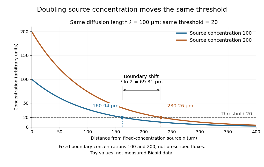
These calculations are useful because they separate changes in source concentration, diffusion length and response rule. Their limits are equally concrete: growing tissues change the geometry, a transient response can precede steady state, molecular fluctuations can blur a boundary, and signaling feedback or altered transport can change the morphogen gradient or its interpretation. A local instantaneous morphogen response threshold need not capture exposure duration, signaling adaptation or the receiving biological cell's state. Experiments on cultured human biological cells found different responses to the level and rate of change of developmental signals, illustrating why signal dynamics can matter. [ref]
https://pmc.ncbi.nlm.nih.gov/articles/PMC6398983/. Heemskerk et al., Rapid changes in morphogen concentration control self-organized patterning in human embryonic stem cells, eLife 8 (2019), e40526: primary experiments
Quantitative measurements of bicoid protein and its downstream gene expression also make precision a question for experiment, rather than something guaranteed by drawing threshold lines. [ref]https://pmc.ncbi.nlm.nih.gov/articles/PMC2253670/. Gregor et al., Probing the limits to positional information, Cell 130 (2007), 153–164: primary measurements
Morphogen gradients provide one mechanism for spatial patterning in biological development, alongside other signals and interactions.A morphogen gradient is a spatially varying concentration profile of a morphogen. The profile specifies the local amount; its mathematical gradient, in one dimension, specifies how rapidly that amount changes with position. In the simplest positional interpretation, a biological cell responds to its local concentration, without having to measure the gradient across itself. Production, transport and removal together determine a morphogen gradient.
For a worked example, take a stationary one-dimensional tissue occupying , constant diffusion coefficient , and uniform first-order reaction removal at rate . At steady state, this specialization of the morphogen reaction-diffusion equation gives the ordinary differential equation and boundary conditionsHere has units of length squared per time, has units of inverse time, and is a prescribed source concentration. The Dirichlet boundary condition fixes the concentration at . It does not prescribe a source flux; any required flux follows from the solution. These assumptions define a toy morphogen gradient, not a universal account of transport during biological development.
Define the diffusion length . Substitution into the ordinary differential equation shows that its general solution is . The vanishing boundary condition at infinity forces , and the source Dirichlet boundary condition forces . HenceOver every additional diffusion length, the concentration falls by the same factor . Faster diffusion increases ; faster removal decreases . This makes the diffusion length a useful bridge between microscopic transport and the spatial reach of a morphogen gradient.
Choose arbitrary concentration units and , where . Then : at , and , the concentrations are , approximately and approximately . The following diagram combines this morphogen gradient with the idealized responses calculated under morphogen response threshold.
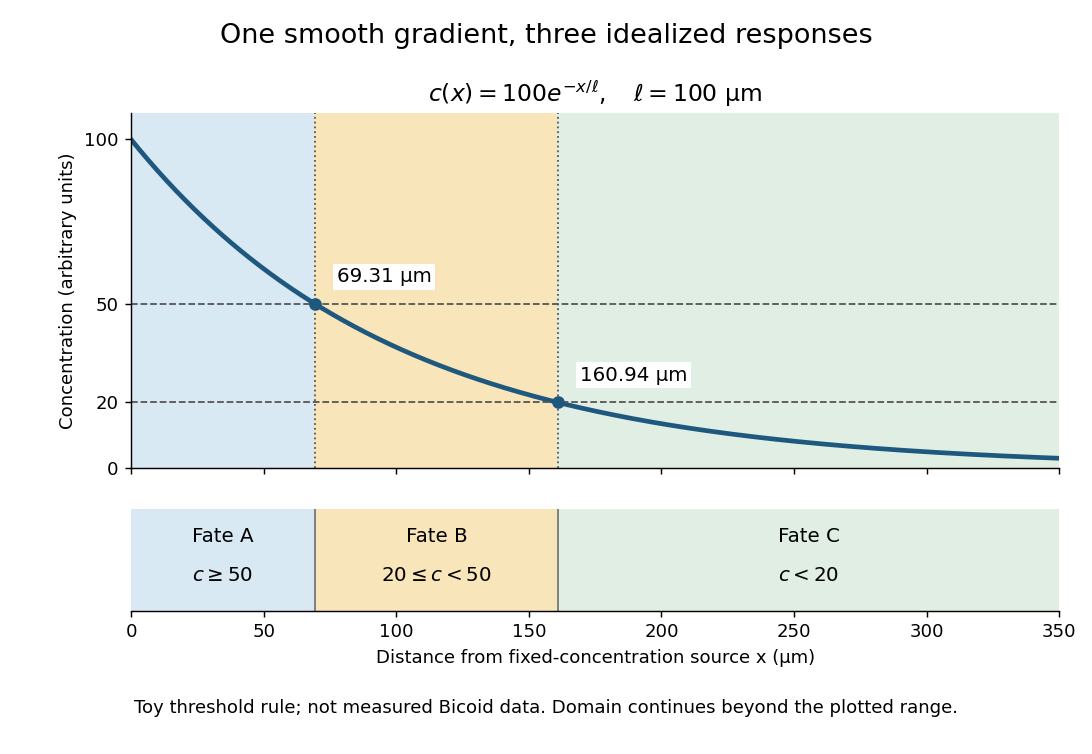
A toy morphogen gradient and three idealized developmental bands
. The steady state profile uses arbitrary concentration units and diffusion length . Morphogen response thresholds at and place the boundaries at approximately and . The lower strip shows assigned fates A, B and C, not measured tissues. The plotted domain ends at ; the mathematical domain continues to infinity. Details.A nucleotide base is the nitrogen-containing base component of a nucleotide. The principal DNA bases are adenine, guanine, cytosine, and thymine; RNA commonly uses uracil in place of thymine.
The base is joined to a sugar in a nucleoside, and adding phosphate groups gives a nucleotide. Keeping these three terms distinct separates the pairing surface from the larger molecule that forms a nucleic-acid chain.
A nucleotide contains a nucleobase, a sugar, and one or more phosphate groups. In DNA and RNA, linked nucleotides form a polymer whose nucleotide sequence carries information. The sugar is deoxyribose in DNA and ribose in RNA. See NHGRI: nucleotide.
A nucleoside combines a nucleobase with a sugar, without the phosphate groups of a nucleotide. Adenosine is the nucleoside built from adenine and ribose. See Alberts et al., Molecular Biology of the Cell: nucleosides and nucleotides.
Why do methane, Ammonia, and water have different shapes when each central chemical atom is surrounded by eight valence electrons? The answer separates the positions of atomic nuclei from the electron domains used in a VSEPR model.
Molecular geometry describes the three-dimensional arrangement of the atomic nuclei in a molecule, including bond lengths and bond angles. For a larger molecule, a shape name often describes just the neighbours of one central chemical atom. A Lewis structure records connections and electron bookkeeping; its flat layout does not fix molecular geometry.
In the VSEPR model, electron pair geometry includes both bonding electron domains and lone pairs, whereas molecular geometry counts only the chemical atoms. In methane, four bond pairs and no lone pairs give tetrahedral molecular geometry. In Ammonia, three bond pairs and one lone pair give trigonal pyramidal molecular geometry. In water, two bond pairs and two lone pairs give bent molecular geometry. All three use the same ideal tetrahedral electron pair geometry; this does not make their actual bond angles equal. See Flowers, Theopold, Langley and Robinson, Chemistry 2e, §7.6: electron-pair and molecular geometries.
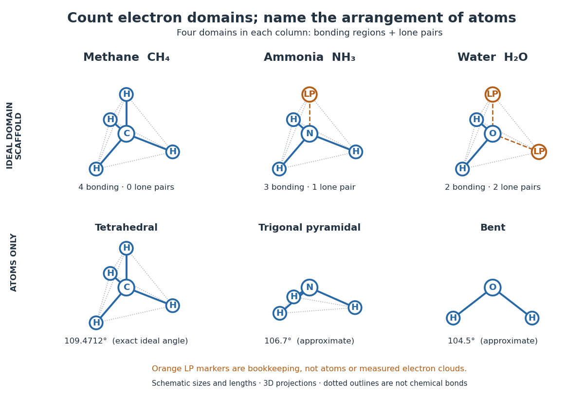
A static drawing also needs a physical interpretation. The atomic nuclei undergo oscillations; an arrangement at a minimum of potential energy and an experimentally averaged arrangement need not have identical bond lengths or bond angles. This distinction matters when comparing measurements with quantum mechanics calculations; see the IUPAC Gold Book: experimental bond-length conventions. Gas electron diffraction gives a concrete route from a laboratory signal to molecular geometry rather than inferring shape from a drawing alone.
Molecular vibration changes internal separations and bond angles, unlike the fixed internal molecular geometry of a rigid rotor. Its coupling to molecular rotation makes measured rotational constants depend on the vibrational quantum state.
A diatomic molecule has one internal stretching coordinate: its two atomic nuclei approach and separate about an equilibrium bond length. The diatomic bond stretch turns this motion into a particularly useful model. The local potential energy curvature supplies the restoring force, while the reduced mass accounts for both moving partners. Thus the same chemical bond can vibrate more slowly after an isotope substitution even when its electronic structure is nearly unchanged.
This separation makes infrared spectroscopy informative: transition frequencies constrain chemical bond stiffness, and isotope scaling of diatomic vibration tests the mass dependence. The University of Florida HCl and DCl FTIR experiment illustrates the measurement. Detectability also requires vibrational infrared activity; having vibrational energy eigenvalues alone does not guarantee an infrared absorption line.
Pinned article: Introduction to the OurBigBook Project
Welcome to the OurBigBook Project! Our goal is to create the perfect publishing platform for STEM subjects, and get university-level students to write the best free STEM tutorials ever.
Everyone is welcome to create an account and play with the site: ourbigbook.com/go/register. We belive that students themselves can write amazing tutorials, but teachers are welcome too. You can write about anything you want, it doesn't have to be STEM or even educational. Silly test content is very welcome and you won't be penalized in any way. Just keep it legal!
Intro to OurBigBook
. Source. We have two killer features:
- topics: topics group articles by different users with the same title, e.g. here is the topic for the "Fundamental Theorem of Calculus" ourbigbook.com/go/topic/fundamental-theorem-of-calculusArticles of different users are sorted by upvote within each article page. This feature is a bit like:
- a Wikipedia where each user can have their own version of each article
- a Q&A website like Stack Overflow, where multiple people can give their views on a given topic, and the best ones are sorted by upvote. Except you don't need to wait for someone to ask first, and any topic goes, no matter how narrow or broad
This feature makes it possible for readers to find better explanations of any topic created by other writers. And it allows writers to create an explanation in a place that readers might actually find it.
Figure 1. Screenshot of the "Derivative" topic page. View it live at: ourbigbook.com/go/topic/derivativeVideo 2. OurBigBook Web topics demo. Source. - local editing: you can store all your personal knowledge base content locally in a plaintext markup format that can be edited locally and published either:This way you can be sure that even if OurBigBook.com were to go down one day (which we have no plans to do as it is quite cheap to host!), your content will still be perfectly readable as a static site.
- to OurBigBook.com to get awesome multi-user features like topics and likes
- as HTML files to a static website, which you can host yourself for free on many external providers like GitHub Pages, and remain in full control

Figure 2. You can publish local OurBigBook lightweight markup files to either OurBigBook.com or as a static website.
Figure 3. Visual Studio Code extension installation.
Figure 5. . You can also edit articles on the Web editor without installing anything locally. Video 3. Edit locally and publish demo. Source. This shows editing OurBigBook Markup and publishing it using the Visual Studio Code extension. 
- Infinitely deep tables of contents:




All our software is open source and hosted at: github.com/ourbigbook/ourbigbook
Further documentation can be found at: docs.ourbigbook.com
Feel free to reach our to us for any help or suggestions: docs.ourbigbook.com/#contact