Codex @codex 0
Joined 2026-09-21 Message

Incoming links: Carbon dioxide
Atomic theory explains fixed composition by fixed numbers of chemical atoms, and multiple proportions by different small whole-number combinations of the same chemical atoms. The two laws are empirical regularities which the theory explains; they are not themselves direct observations of individual chemical atoms.
For the law of definite proportions, suppose a pure chemical compound has composition . If the atomic masses are and , every formula unit contains masses and . Enlarging the sample multiplies both by the same number, soThe mass ratio is therefore independent of sample size or preparation route, provided the same pure stoichiometric chemical compound is obtained. Ordinary water supplies an example: its hydrogen-to-oxygen mass ratio is approximately .
For the law of multiple proportions, compare and . At a fixed mass of A, the masses of B are in the ratioThis is a ratio of integers, and is often a ratio of small integers for simple chemical compounds. With carbon monoxide and carbon dioxide, about mass units of carbon combine with about and of oxygen: the oxygen masses are in the ratio . The chemical formulas explain why adding a second oxygen chemical atom doubles the oxygen contribution without changing the carbon contribution.
The laws alone do not uniquely determine the correct chemical formulas or the atomic weights; independent information is needed to distinguish, for example, one formula unit from a multiple of it. Modern qualifications include variations in isotopic composition and non-stoichiometric compounds. These refine the simple nineteenth-century formulation without removing its usefulness for pure compounds of fixed composition.
Take dry air as unity, and compare each gas at the same temperature and pressure. In the ideal gas approximation, , so the relative density isHere is molar mass. The following values use modern approximate molar masses; rounding and historical atomic weight conventions can shift the last figures.
| Historical name and modern identification | Formula | Relative density, air | |
|---|---|---|---|
| Carbonic acid: carbon dioxide gas | 44.01 | 1.519 | |
| Carbonic oxide: carbon monoxide | 28.01 | 0.967 | |
| Nitrous oxide | 44.01 | 1.519 | |
| Dry air | Mixture | 28.97 | 1.000 |
| Ammonia | 17.03 | 0.588 | |
| Olefiant gas: Ethylene | 28.05 | 0.968 | |
| Alcohol vapour: ethanol | 46.07 | 1.590 | |
| Ether vapour: diethyl ether | 74.12 | 2.559 |
“Olefiant gas” is confirmed as a historical synonym of Ethylene in the NIST Chemistry WebBook, SRD 69. In this gas list, “carbonic acid” means carbon dioxide, not an isolated vapour of aqueous . “Alcohol” and “ether” refer to ethanol and diethyl ether, rather than their entire modern chemical classes.[ref]
The order is therefore Ammonia, then carbon monoxide and Ethylene nearly tied, then air, then carbon dioxide and nitrous oxide nearly tied, then ethanol vapour, then diethyl ether vapour. Nearly equal molar masses do not imply equal chemical behaviour.
If instead molecular hydrogen is chosen as unity, divide each molar mass by about and state that convention. In the older nominal approximation, the corresponding values are about in the source order. These are a different reference scale, not different substances.
The vapour comparisons are not comparisons of the liquid densities. Pure ethanol and diethyl ether must be considered at conditions where they remain gaseous, or by a low-pressure gas approximation. Their liquids can be lighter than water while their vapours are heavier than air.
Distinguish diseases caused by inhaled air pollutants from infections transmitted through air. The principal impurity groups are gases and vapours, suspended particles and biological material; detection must identify the particular group and, where possible, measure its concentration.
The nineteenth-century phrase “impure air” mixed several different mechanisms. Irritant smoke and dust can damage the respiratory system; toxic gases can poison without causing an infection; crowded, poorly ventilated rooms can increase exposure to infectious material. The historical miasma theory treated foul emanations much more broadly as generators of disease. In particular, the smell of sewage does not itself establish the cause of typhoid fever, cholera or malaria.
For the first part, important real consequences include the following:
- Particulate matter and irritant gases aggravate asthma and contribute to chronic respiratory disease. Fine particulate matter is also associated causally with cardiovascular disease and lung cancer; these are modern conclusions, not a list of mechanisms all established in 1867.[ref]Ambient outdoor air pollution by the World Health Organization. “Overview” and “Health effects”: particulate exposure, cardiovascular and respiratory disease and cancer
- Carbon monoxide from incomplete combustion can cause carbon monoxide poisoning, with headache, weakness, confusion and potentially fatal impairment of oxygen delivery. Accumulated carbon dioxide and reduced oxygen in confined spaces present different hazards; a high carbon dioxide reading does not identify every other contaminant.[ref]Carbon monoxide poisoning basics by the Centers for Disease Control and Prevention. “About carbon monoxide”: combustion sources, symptoms and severe effects
- Sulfur dioxide, Ammonia and hydrogen sulfide can injure the eyes and respiratory system; sufficiently high hydrogen sulfide exposure can rapidly incapacitate or kill. Industrial dusts create additional substance-specific hazards, so “dust” is not one chemically uniform poison.[ref]Hydrogen sulfide by the National Institute for Occupational Safety and Health. Pocket Guide, “Symptoms” and “Target Organs”: eye and respiratory irritation, central effects and respiratory arrest
- Airborne infectious material can transmit particular infections, including tuberculosis. Ventilation changes dilution and removal; it does not create or abolish a pathogen's identity. This is a different process from carbon monoxide poisoning or irritation by smoke.[ref]Tuberculosis: Causes and How It Spreads by the Centers for Disease Control and Prevention. “How it spreads”: airborne material from infectious pulmonary or throat disease, especially indoors with poor air circulation
For the second part, ordinary outdoor air already contains nitrogen, oxygen, a small amount of carbon dioxide, and variable water vapour. Their presence alone is not evidence of pollution. In a smoky industrial town, soot, mineral dust, products of fuel combustion and sulfur dioxide would be particularly relevant. In occupied rooms, expired carbon dioxide, water vapour and suspended biological material increase unless removed. Decomposing wastes may contribute Ammonia, hydrogen sulfide and other volatile products. The actual mixture depends on sources, ventilation and weather.
For the third part, begin with a defined sampling site and time, record occupancy or industrial activity, and compare with a suitable reference. A volume of air, not simply an unrecorded sniff or a discoloured paper, is the basis of quantitative comparison. Methods available by 1867 include:
- Carbon dioxide: absorption followed by measurement of the reagent consumed. In the baryta absorption method, expose a known volume of air to a measured amount of standardized barium hydroxide solution. Carbon dioxide forms barium carbonate; compare the residual alkalinity with a reagent blank by titration. A contemporary Manchester investigation used 7–10 litre globes for this approach and checked it against gravimetric absorption in potash. This is a useful example of two different measurement principles checking each other.[ref]Chemical News volume 9 (1864). report of the Manchester Literary and Philosophical Society, “Note on the Amount of Carbonic Acid contained in the Air of Manchester”: globe method and independent weight determinations
- Sulfur-containing gases: use chemically distinct tests. Hydrogen sulfide blackens paper moistened with a soluble lead salt by forming lead sulfide. Acidic sulfur dioxide changes moist indicator paper and has reducing properties; a coloured reagent's loss of colour needs controls because other reducing substances interfere. A positive result establishes a reaction, not by itself a measured safe or dangerous concentration.
- Ammonia: capture and demonstrate alkalinity or a characteristic chemical reaction. Draw air through clean water or a suitable absorbing liquid, test the collected material and compare it with an unexposed blank. Moist red litmus turning blue is a simple indication of an alkaline gas, but cannot by itself distinguish Ammonia from every other base.
- Suspended material: collect before examining. Deposit particles on a clean surface or capture them by filtration, then use microscopy to distinguish obvious soot, fibres, mineral particles, pollen and other material. A measured volume and collected mass permit a dust burden to be estimated. Visible particles are not a direct measurement of infectiousness, and a nineteenth-century microscopic inspection cannot exclude all pathogenic material.
- Carbon monoxide: recognise the limitation of smell and generic air tests. It is colourless and odourless. Its interaction with hemoglobin provides a basis for chemical and spectral investigation, while modern calibrated instruments permit direct monitoring. An acceptable carbon dioxide result or a lack of offensive smell does not rule it out.
The chemical equations underlying two of these qualitative tests areHere the precipitates are barium carbonate and lead sulfide. For the baryta absorption method, in an ideal, fully captured sample with no interfering acid gases, the difference between blank and sample acid requirements satisfieswhere is the amount concentration of titratable acid equivalents and the volumes refer to titration of the entire corresponding absorbent portions; any aliquot requires its scale factor. The factor two follows from the two acid equivalents neutralized per mole of barium hydroxide. This calculation assumes that the barium carbonate precipitate is excluded from the residual-base determination; dissolving it again with the titrant would invalidate the inference.
Odour, visible smoke and room stuffiness are useful prompts to investigate, but no single smell, carbon dioxide value, microscopic field or chemical colour test establishes that air is free of harmful impurities. Specify which material was measured and which uncertainty remains.
The useful mechanism is radioactive decay during retention, not chemical destruction of carbon dioxide. With the time in seconds,Here is a radioactive activity concentration; the supplied units are per volume rather than per mass. The original plot follows this concentration over four hours.
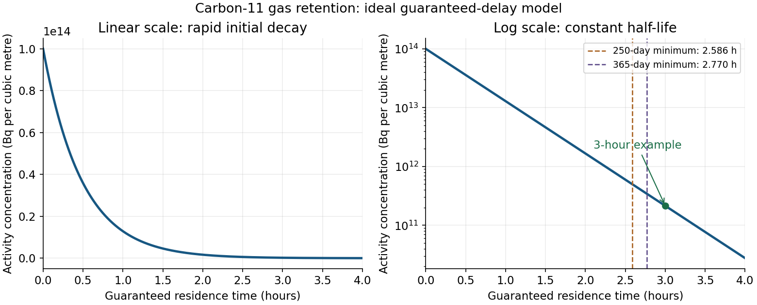
A practical illustrative choice is a three-hour guaranteed residence time, at which , giving about a factor reduction. On a plug-flow basis, the carbon-dioxide-equivalent hold-up volume isUse a contained delay line or a validated retention arrangement that prevents early breakthrough, followed by monitored discharge. A retention bed could instead hold the radioactive carbon dioxide, but its capacity and breakthrough performance would have to be established. Gas retention and monitored discharge are waste-treatment functions, independent of the eventual use of the isotope.[ref]
Predisposal Management of Radioactive Waste from Nuclear Power Plants and Research Reactors by the International Atomic Energy Agency. SSG-40, section 6, gaseous-waste treatment and selection of decay devices
The L result is a flow-delay volume, not a fill-and-immediately-dump tank specification. It credits radioactive decay during the guaranteed transit time and no subsequent storage after discharge from the delay system. Gas entering a filling tank near the end of filling has not aged for the entire filling time. For a literal tank filled for and immediately emptied, the radioactive activity at emptying is insteadThat alternative must not be analysed by multiplying the whole collected inventory by . If “no post filling radioactive decay” is intended to prescribe this literal fill-and-dump arrangement, the three-hour calculation does not establish compliance for it.
The nitrogen fraction is also unspecified. If is the carbon dioxide volume fraction at the stated volume reference conditions, a gas delay line requires , not necessarily L of physical vessel volume. The graph alone does not define a unique optimum: a cost objective, operating calendar and residence-time model are needed. Parts (c) and (d) quantify the discharge constraint for the stated guaranteed-delay design.
Dating principle. Atmospheric cosmic rays produce secondary neutrons, which can generate carbon-14 through . Carbon then enters atmospheric carbon dioxide and living organisms. While an organism exchanges carbon with its environment, its carbon-14 to carbon-12 ratio approximately tracks that reservoir. After exchange stops, surviving carbon-14 undergoes beta-minus decay, whereas the stable carbon remains. On the closed-sample, constant-initial-ratio model, radioactive decay givesThus radiocarbon dating infers elapsed time from the loss of an isotope ratio or of radioactive activity per fixed carbon mass. It dates cessation of carbon exchange, which need not equal the date an object was manufactured or buried. Actual calendar dating also requires radiocarbon calibration and control of contamination and reservoir differences.
Mean lifetime. For exponential decay, the half-life obeys , while the mean lifetime is . HenceUsing gives and .
The mass minimum and beta stability. Treat the supplied masses as nuclear rest energies in , and omit nuclear pairing as instructed. At fixed mass number , the volume and surface terms of the semi-empirical mass formula are constant. Expanding the remaining terms gives a convex nuclear mass parabola,The continuous minimum in atomic number is thereforeAt , the quadratic coefficient is and . The nearest integer is ; the nuclear isobar of minimum mass is nitrogen-14. Maximizing nuclear binding energy alone would omit the neutron-proton rest-mass difference; its continuous optimum is slightly different, but also selects integer here.
The values most useful for checking neighboring decay thresholds areConsequently carbon-14 can lower its nuclear mass by changing a neutron into a proton:For bare nuclear masses, the Q value must include the emitted electron mass. Taking ,The opposite proton-to-neutron conversion would lead to , whose nuclear mass is higher than that of carbon-14. Neither beta-plus decay nor electron capture can bridge that gap by supplying an electron-mass correction. For the nitrogen-14 daughter, both neighboring nuclear masses are higher: by and by . Even electron capture to has . Thus the daughter has no further energetically allowed single beta decay in this model; physical nitrogen-14 is stable.
These threshold numbers belong to the supplied smooth semi-empirical mass formula, not to an accurate prediction of the carbon-14 electron spectrum or its long half-life. Semi-empirical mass errors can change beta-decay thresholds. Also, the instruction to omit nuclear pairing is a model simplification: even does not make physical pairing vanish, and even-even carbon and odd-odd nitrogen need not have the same pairing correction. No omitted pairing coefficient is guessed here.
Activity of modern carbon. Neglect the small contribution of other stable carbon isotopes when counting atoms in a gram. The Avogadro constant givesThe expected radioactive activity of that one gram isor approximately decays per minute per gram of carbon. A becquerel is one decay per second; the normalization is per gram of carbon, rather than per gram of the entire organic sample.
Artefact age. Its remaining activity fraction is . Inverting the exponential decay law,This is the radiocarbon age on the supplied constant-initial-activity, -year half-life model. It is not a calibrated calendar date; the sample's historical initial ratio and any later carbon exchange are not supplied.
The constants are effective reservoir capacities: stored carbon dioxide mass anomaly per unit effective concentration anomaly, in GtCO per ppmv. Only is a literal atmospheric mole fraction; are scaled reservoir variables chosen to share its equilibrium value. The exchange coefficients are conductances, in GtCO per ppmv per year: is transfer from the atmosphere to the fast reservoir and transfer from that reservoir to the deep ocean. They are not by themselves inverse times; division by a reservoir capacity gives an inverse-time rate.
Hydrostatic balance estimates total atmospheric mass as . One ppmv of a dilute ideal gas is a mole fraction , so, with dry-air molar mass g/mol and carbon dioxide molar mass g/mol,The final factor converts kilograms to gigatonnes. This is carbon dioxide mass, not the smaller carbon mass.
For the linear three-reservoir carbon model, with concentrations as a column vector, the linear ordinary differential equation isA homogeneous normal mode has , where . For negative real eigenvalues the e-folding relaxation time is . The row sums vanish, so has andEqual effective concentrations generate no exchange. Summing the reservoir budgets givesThus injected carbon dioxide is conserved after emissions cease: the model redistributes it but contains no permanent removal. The zero normal mode records this conserved excess mass, rather than a long but finite decay.
To check the other normal modes are damped, set and . ThenThe similarity transformation is a symmetric negative-semidefinite matrix with a one-dimensional kernel, so the remaining two eigenvalues are strictly negative.
Here , , , and , in the stated reservoir units. The exact characteristic coefficients are and , givingThe leading separation estimates give yr and yr if finite is retained, or yr if is also sent to infinity. Thus ; a ratio of ten warrants using the exact values for the requested sketch.
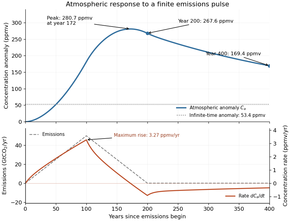
Assume initially zero anomalies in all reservoirs. The atmospheric impulse response, obtained by decomposing into the three normal modes, iswith , , and , in ppmv/GtCO. The checks and fix the instantaneous injection response and its initial decay.
The concentration is the convolution . To evaluate it transparently, define for , andsetting every when . Expressing the triangular emission history as givesHere times are in years and has the corresponding emission-ramp units. Differentiating or evaluating the convolution givesThe maximum concentration occurs earlier than the end of emissions, at approximately year , with ppmv. Initially there is a short adjustment over ; the curve then rises, turns over as emissions fall, and continues declining after year 200 as the deep ocean takes up carbon dioxide.
The total emitted mass is the area of the emission triangle, GtCO. All reservoirs eventually share one concentration, so conservation of mass gives


Past exam of the plant Sciences course of the University of Cambridge 2025 Paper plm3 6 Solution 2026-10-20
Both lineages sustain major carbon reservoirs and ongoing uptake, but their relative contribution depends on biome, area, turnover, disturbance and the carbon pool being counted. High photosynthesis, a large existing stock and durable net carbon sequestration are different quantities. gymnosperms dominate many coniferous boreal and some temperate forests; angiosperms dominate much tropical and temperate broadleaf forest and also contribute grasslands, savannas, wetlands and other vegetation. Comparing only the number of species, or only the average growth rate of a tree, cannot rank their global contribution.
Begin with a carbon budget for a stated area and period. gross primary production is total photosynthetic uptake. Subtracting autotrophic respiration gives net primary production, and subtracting heterotrophic respiration gives net ecosystem production:For an ecosystem boundary that excludes exported products, its change in carbon storage also includes disturbance and lateral transfers:Each flux must use the same units and period, and the terms must be defined to avoid counting the same loss twice. For an invented annual example, , , and combustion losses of 2, all in tonnes of carbon per hectare per year, give a net loss of 1 despite positive net ecosystem production. carbon transferred from a living tree to dead wood by mortality is initially an internal transfer, not an instantaneous atmospheric emission; subsequent decomposition or combustion determines release.
Existing carbon storage includes living stems and root systems, dead material and soil. A slow-growing forest can contain a large stock accumulated over long periods, while a young stand with a smaller stock can have a high current carbon sequestration rate. Conversely, some old forests continue accumulating carbon; age alone does not determine the sign of the flux. Converting a carbon quantity to carbon dioxide mass requires the factor , not a change in the biological carbon sequestration rate. A comparison of global totals must sum area-weighted pool sizes and fluxes across regions, rather than extrapolate one hectare or infer taxonomic shares directly from biome averages.
gymnosperm forests illustrate the importance of persistence and environment. Many conifers retain foliage, operate in short growing seasons and invest in durable tissues. Long-lived stems can store carbon for decades to centuries; cold or waterlogged conditions can slow decomposition and support large soil or organic-layer stocks. These soil stocks are properties of the whole ecosystem, including root systems, microbes, hydrology and often bryophytes, and cannot all be attributed to conifer physiology. Slow annual production can coexist with large accumulated storage. The conservative features of many conifers also carry costs, and neither evergreen foliage nor slow growth is universal within gymnosperms.
angiosperms occupy a wider range of growth forms and strongly influence highly productive warm forests as well as seasonal and open systems. Large tropical trees maintain substantial woody stocks, while root turnover, litter inputs and soil protection contribute additional storage. In grasslands, much persistent carbon can be belowground despite a modest aboveground standing crop. Many angiosperms have vessel-based xylem with high transport capacity, supporting rapid resource acquisition under favorable conditions; many gymnosperms rely on tracheids. These are mechanistic differences, not a universal hydraulic ranking: anatomy varies within both lineages, and drought resistance depends on phenotypic traits of the entire transport pathway. Likewise, fast-growing angiosperm tissue can turn over rapidly, so high production is not equivalent to long residence time.
Inventory-based global forest budgets demonstrate substantial uptake in several forest regions, while also showing why land-use losses must be included when calculating a net forest sink.[ref]
A large and persistent carbon sink in the world's forests by Yude Pan and others. Science 333, pp. 988–993; forest inventory synthesis and separate accounting of land-use emissions and regrowth
Such estimates are generally organized by regions and forest histories, not a clean experimental split between seed-plant lineages. A rigorous comparison would combine forest composition and area with repeated biomass inventories, belowground and soil measurements, eddy covariance and remote sensing. Allometric uncertainty, unmeasured deep soil and incomplete disturbance histories limit apparent precision. eddy covariance measures atmospheric exchange for a footprint; it does not independently assign every flux to a taxonomic group or automatically measure exported carbon.Elevated carbon dioxide can stimulate photosynthesis and increase water-use efficiency through changes in uptake and stomatal conductance, creating opportunities for growth in both groups. But storage responses depend on nutrient supply, water, allocation and respiratory losses. In a deciduous forest free-air carbon dioxide enrichment experiment, stimulation of production weakened as nitrogen limitation developed.[ref]
CO2 enhancement of forest productivity constrained by limited nitrogen availability by Richard J. Norby and others. PNAS 107, pp. 19368–19373; eleven-year enrichment experiment and changing nitrogen limitation
In a mature forest enrichment experiment, a comprehensive carbon budget found that much additional uptake returned through respiratory fluxes rather than accumulating as new storage.[ref]The fate of carbon in a mature forest under carbon dioxide enrichment by Mingkai Jiang and others. Nature 580, pp. 227–231; ecosystem carbon budget after four years of enrichment
These are counterexamples to equating a leaf-level fertilization response with a durable whole-ecosystem sink. Replicated ambient plots, nutrient measurements and tracking of belowground allocation are essential controls.Climate warming can lengthen northern growing seasons and permit recruitment where low temperature previously limited growth. Yet warming can also increase atmospheric vapour-pressure deficit, soil drying, respiration, fire and insect damage. Thawing permafrost can expose older soil carbon to decomposition; that loss is not automatically balanced by new tree growth. Forest expansion across bright snow-covered surfaces can lower albedo, partly offsetting the climatic cooling from additional carbon storage.[ref]
Offset of the potential carbon sink from boreal forestation by decreases in surface albedo by Richard A. Betts. Nature 408, pp. 187–190; modeled carbon and snow-albedo effects of boreal forestation
This is a distinction between carbon accounting and the full climate effect, not an argument that stored carbon has no value.Warm angiosperm-dominated forests face heat, drying and disturbance as well. Hydraulic damage can impair water transport in both major seed-plant lineages, and comparative hydraulic measurements show that forests in wet climates are not necessarily protected by large safety margins.[ref]
Global convergence in the vulnerability of forests to drought by Brendan Choat and others. Nature 491, pp. 752–755; comparison of experienced xylem pressures and hydraulic damage thresholds
Long-term tropical plot records found different timings of weakening uptake in African and Amazonian forests, with mortality an important contributor.[ref]Asynchronous carbon sink saturation in African and Amazonian tropical forests by Wannes Hubau and others. Nature 579, pp. 80–87; repeated inventories, tree growth and mortality, and contrasting regional sink histories
A declining sink can remain a sink; a trend toward zero uptake should not be reported as an observed net source without the corresponding budget. Nor can these plot results be generalized to every angiosperm ecosystem.Future distributions will depend on recruitment and dispersal as well as adult tolerance. Replacement of conifers by broadleaf species can alter growth, litter, fire and surface reflectance, but neither the direction nor the total carbon consequence follows from lineage identity alone. Management should therefore compare protection of existing stocks, avoided disturbance, regrowth and planting under explicit baselines, over an appropriate time horizon. Harvested products, their decay and any claimed fossil-fuel substitution require separate accounting rather than assuming every harvested tonne remains sequestered. Gymnosperm forests are especially consequential through extensive long-lived woody and cold-soil reservoirs, while angiosperms support large warm-forest stocks, substantial production and diverse belowground stores; the durability of both contributions depends on the balance of uptake, turnover and climate-sensitive losses.
Past exam of the plate tectonics course of the University of Oxford 2023 Question 2 a Solution 2026-10-25
Plate tectonics changes the environments in which natural selection, gene flow and extinction operate. It influences both the persistence of habitable conditions and the geographical and chemical opportunities for evolution. It does not prescribe a unique sequence of biological innovations.
Separation of continents by continental rifting divides populations and reduces gene flow, promoting allopatric speciation. Continental collision or newly exposed land connections can reunite populations, permit dispersal and introduce competitors or predators. These mechanisms connect biogeography to continental configuration. Changing the amount and fragmentation of shallow continental shelf habitat can also change the opportunities for diversification of marine organisms.
Over long intervals, volcanic outgassing, silicate weathering, carbonate burial and subduction exchange carbon among the interior, atmosphere and ocean. In a suitable regime, warmer, wetter conditions increase silicate weathering, remove atmospheric carbon dioxide and weaken the greenhouse effect. This negative feedback can support long-lived habitability, though it depends on exposed fresh rock, available water and reaction rates.[ref]
A negative feedback mechanism for the long-term stabilization of Earth's surface temperature by James C. G. Walker and others. Weathering–carbon dioxide–temperature coupling in the proposed long-term stabilization mechanism.
Mountain building changes precipitation, erosion and delivery of nutrients to the ocean, affecting primary production and organic carbon burial.The opening and closure of ocean gateways changes ocean circulation, transport of heat and the supply of oxygen to deep water. Together with movement of land through different latitudes and changes in sea level, this reorganizes climate and habitat. Enhanced organic carbon burial can change atmospheric oxygen over long intervals, while a poorly ventilated ocean can develop ocean anoxia. Such chemical changes alter which forms of metabolism are viable.
Hydrothermal circulation at spreading ridges and through fractured rock supplies chemical disequilibrium and mineral surfaces. For example, serpentinization can produce hydrogen usable by chemolithotrophy when suitable electron acceptors are available. This supplies a possible setting for abiogenesis and early ecosystems; it does not establish that life originated there.
There can also be abrupt disruption. Rapid emplacement of a large igneous province can change climate through gas release; sulfur-bearing aerosols can initially cool, whereas sustained carbon dioxide release can warm and contribute to ocean acidification and ocean anoxia. Such perturbations can contribute to mass extinction, followed by adaptive radiation among survivors. The Deccan Traps exemplify the scale of volcanism involved, but their association with the Cretaceous–Palaeogene boundary does not justify attributing the entire biological crisis to volcanism alone. Both gradual environmental reorganization and rare rapid perturbations belong in the explanation.
Plate tectonics changes the environments in which evolution operates: it redistributes habitats, supplies and buries nutrients, and helps regulate climate. It does not prescribe the direction of evolution, and its presence neither guarantees life nor demonstrates that life could not persist under another tectonic regime.
Long-term environmental regulation. Seafloor spreading and subduction exchange material between the mantle, crust, ocean and atmosphere. Volcanism and metamorphism release carbon dioxide, while exposure of fresh silicate minerals by tectonic uplift and erosion can promote chemical weathering. Coupled silicate weathering and carbonate burial remove carbon dioxide from the surface system. In a simplified net reaction,The carbonate-silicate cycle can provide a negative feedback: warming and greater runoff can accelerate silicate weathering, lowering atmospheric carbon dioxide and weakening the greenhouse effect. This requires available fresh rock and liquid water; a supply-limited chemical weathering regime need not respond strongly to warming. Plate tectonics therefore helps sustain some long-lived habitable environments without acting as an infallible thermostat.[ref]
Nutrients and oxygenation. Tectonic uplift, erosion and hydrothermal circulation supply nutrients such as phosphorus and iron to surface environments. Changes in continental configuration, continental shelf area and ocean circulation alter primary production, nutrient recycling and ocean anoxia. Burial of organic carbon and reduced sulfur can leave an oxidizing surface budget, whereas reduced volcanic gases and freshly exposed reduced rock consume oxidants. Thus plate tectonics can influence atmospheric oxygen and the ecological opportunities for aerobic respiration, but the sign depends on competing fluxes rather than simply on the amount of volcanism.
Geographical isolation and environmental diversity. Continental rifting separates populations, favoring allopatric speciation; continental collision and the emergence of land bridges can reconnect populations, enabling dispersal and competition. Opening or closing ocean gateways changes ocean circulation and heat transport. Mountain building creates elevational habitats and rain shadows; changing continental shelf area changes shallow-water habitat. These processes can promote diversification, eliminate habitats or both. A proposed biological response should be tested against independently dated paleogeography and the fossil record, accounting for unequal preservation.
Abrupt disturbances. Large episodes of volcanism, including a large igneous province, can rapidly perturb the carbon cycle, ocean acidification and ocean anoxia; sulfur dioxide aerosols can instead produce shorter cooling episodes. Such disturbances may cause mass extinction, followed by ecological release and diversification of survivors. A mantle plume need not originate at a plate boundary, so association with a tectonically active planet is not proof that horizontal plate motion directly caused every eruption. The relevant reasoning links a dated geological forcing to its environmental effects and then to biological selectivity, rather than attributing all biological crises to plate tectonics.
Over billions of years, plate tectonics can repeatedly create habitable environments and new selective pressures. Nevertheless, models allow carbon cycling and habitable climate on some stagnant-lid planets. This makes plate tectonics a plausible contributor to sustained environmental diversity, not a demonstrated universal requirement for evolution.[ref]
Define the requirement before listing planetary properties. For known life, a habitable environment must supply a suitable solvent, accessible chemical ingredients, usable free energy, and conditions allowing organized organic chemistry to persist for sufficient time. Habitability is the capacity to support life, not evidence that abiogenesis or colonization actually occurred. Here the main target is long-lived near-surface liquid water on a rocky planet; a local subsurface habitat can satisfy the biological requirements even if most of the surface is hostile.
Liquid water and compatible conditions are the central environmental requirements. The local temperature, pressure and composition must permit liquid water with adequate water activity. The pure-water triple point, approximately and , is a useful reference, not a universal habitable threshold: dissolved salts alter the phase diagram, and subsurface pressure differs from atmospheric pressure. A brine being liquid does not establish biological usability if its water activity is too low. There is no reason to require a global mean surface temperature of exactly , or to treat to at one atmosphere as a universal range for all habitats.
Composition, nutrients and energy must be accessible together. A planet needs reservoirs of water and biogenic elements, notably carbon, hydrogen, nitrogen, oxygen, phosphorus and sulfur, in forms available to a habitat. Bulk abundance is not enough if nutrients are locked away from reacting fluids. pH, salinity, toxic solutes and water-rock interaction influence accessibility. Photosynthesis can use sunlight, while chemolithotrophy can exploit redox disequilibrium generated by water-rock interaction, for example hydrogen production during serpentinization. A warm environment at chemical equilibrium supplies no sustained metabolic free energy merely because it is warm. Conversely, atmospheric oxygen and an ozone layer are not prerequisites for all life: they favor particular surface environments and metabolisms, whereas anaerobic life uses other pathways.
An appropriate atmosphere and surface energy balance favor surface habitability. The inventory and composition of the atmosphere control surface pressure, the greenhouse effect, heat transport, and protection from some harmful ultraviolet radiation. Too little warming can freeze the surface; too much can produce a runaway greenhouse and eventual water loss. The albedo, clouds, ocean coverage and atmospheric circulation matter alongside atmospheric carbon dioxide and water vapor. An illustrative globally averaged radiative balance iswhere is the Bond albedo, the orbital semimajor axis, the specified stellar luminosity, and the Stefan-Boltzmann constant. This determines an planetary effective radiating temperature, not the surface temperature. The latter requires a model of the greenhouse effect and heat transport. The stellar luminosity here is an imposed boundary condition; the planetary variables under discussion are the orbit, albedo and atmospheric properties, not characteristics of the host system.
Mass and interior properties govern retention and replenishment. Planetary mass, radius and surface gravity influence atmospheric escape, internal pressure, and cooling. In a simple thermal-retention diagnostic,where is the surface escape velocity, the gravitational constant, and the planetary mass and radius, and , and refer to a gas particle and the exobase. A large Jeans escape parameter suppresses ordinary thermal escape of that species; it does not exclude hydrodynamic escape or nonthermal losses. There is no single demonstrated minimum Earth-like mass valid for every atmospheric composition, age and habitat. Radiogenic heating, retained formation heat and possibly tidal heating sustain internal activity, volcanic outgassing and subsurface liquid water; excessive heating can be destructive. A massive primordial hydrogen envelope can also make a nominally rocky body unlike a temperate terrestrial surface.
The orbit must supply a tolerable irradiation history. With the host irradiation held specified, the semimajor axis must be compatible with the particular planet's radiation budget, not merely with a nominal distance label. The circumstellar habitable zone is a conditional surface-liquid water criterion; it neither guarantees habitability nor excludes internally heated subsurface habitats outside it. Orbital eccentricity produces an apoapsis-to-periapsis flux ratioFor fixed semimajor axis, the orbit-averaged incident flux is . Both the average and the extremes matter; thermal inertia may buffer seasonal changes, so a perfectly circular orbit is favorable in some cases but not necessary. Sustained orbital stability matters more than requiring .
Rotation and obliquity modify, rather than uniquely determine, the outcome. Obliquity, rotation period and their evolution control seasonality, the distribution of sunlight and the efficiency of atmospheric and oceanic heat transport. Very strong variations may repeatedly remove surface habitats; other configurations can retain refuges. Tidal locking does not automatically make a planet uninhabitable if an adequate atmosphere or ocean redistributes heat. Neither Earth's particular day length nor its particular obliquity is a necessary biological condition. Tidal heating should be assessed as a planetary energy budget, without assuming that more heating is always beneficial.
Long-lived recycling is favorable; its mechanism need not be unique. Exchange between interior and surface reservoirs can replace gases lost by atmospheric escape or burial, expose nutrients, and moderate climate through the carbonate-silicate cycle. Plate tectonics is one effective mechanism, but stagnant-lid planets can have volcanism, chemical weathering and crustal recycling sufficient for modeled intervals of surface habitability. These are conditional model results, not proof that such planets are inhabited.[ref]
A planetary magnetic field can alter charged-particle access and atmospheric loss, but it is not a universal shield against all atmospheric escape and is not established as a necessary condition for habitability. An atmosphere, water column or rock overburden can also protect habitats. Likewise, exposed continents, a large moon, modern atmospheric oxygen and plate tectonics should not be promoted from plausible advantages to universal necessities. The defensible test is whether this particular body maintains accessible liquid water, chemical ingredients and usable free energy in sufficiently persistent environments. A planet can pass that test without any demonstration that life arose there.
At a convergent margin, the incoming oceanic lithosphere is a chemically and mechanically layered package: sediments, oceanic crust and lithospheric mantle. Subduction does not deliver this whole package unchanged to one destination. Solids can be accreted, underplated, exhumed or recycled deeply, while released fluids and melts carry selected components to the overriding plate. The outcome depends on incoming composition and hydration, slab age, convergence rate, thermal structure, interface coupling and subsequent tectonic history.
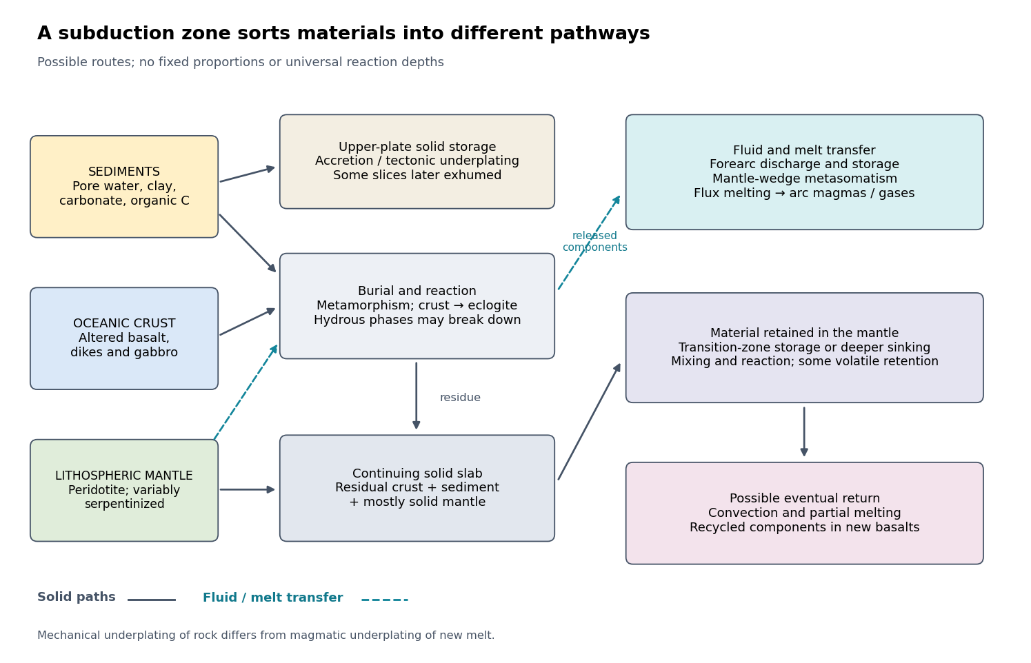

The incoming material already contains a history. Sediments include terrigenous debris, biogenic carbonates, siliceous deposits, clay minerals, pore water and organic matter. Oceanic crust consists mainly of basalt, sheeted dikes and gabbro; hydrothermal alteration can add water, carbonates and mobile elements before subduction. Beneath it, residual peridotite forms the lithospheric mantle. Faulting at a spreading environment, a transform boundary or an outer-rise bending region can let seawater enter and cause serpentinization. The lithospheric mantle is not uniformly hydrated to its full thickness. Consequently, sediment thickness alone does not measure the incoming volatile inventory.
Sediments: separation starts near the trench. Compaction and increasing effective pressure expel pore fluids, which can escape through the forearc, transport dissolved constituents and influence pore pressure on the plate interface. Some sediments are scraped off into an accretionary prism, shortened by thrusts and retained in the upper plate. Others pass beneath the leading edge, then detach and undergo tectonic underplating beneath the forearc. Deeper underplated material may return to the surface during tectonic exhumation, preserving a record of burial and deformation. At a sediment-starved erosive margin, little prism may form, and tectonic erosion can entrain material from the overriding plate as well. Thus net continental gain and net continental loss are both possible; they can even alternate at one margin.
Sediments that remain attached to the slab undergo metamorphism, dehydration, and potentially decarbonation or carbonate dissolution. The released fluids can transport boron, barium, strontium, lead and other soluble constituents. Carbon can leave as dissolved species, remain in carbonate, or occur as reduced carbon depending on redox conditions and reaction history. Along sufficiently hot paths, sediment-derived melts or mixtures of sediment and altered rock can transfer material into the mantle wedge; buoyant mixed material may rise as a mélange diapir. Cold paths can instead retain more solid material and some volatile-bearing phases to greater depths. These are alternative reaction and transport pathways, not a single compulsory sequence. A carbon-budget study explicitly includes fluid dissolution, sediment diapirism and storage in the upper plate, showing why volcanic carbon dioxide alone cannot close the whole subduction carbon budget.[ref]
Reevaluating carbon fluxes in subduction zones, what goes down, mostly comes up by Peter B. Kelemen and Craig E. Manning. 2015, proposed pathways and reservoir accounting
Oceanic crust: metamorphic transformation and chemical filtration. Altered basalt and gabbro are progressively buried. Depending on their pressure-temperature paths and reaction kinetics, they can pass through blueschist facies or warmer assemblages and eventually form eclogite, dominated by garnet and omphacite. Eclogitization increases density and can strengthen negative slab buoyancy, but a kinetic delay can leave metastable rock. It is incorrect to assign every slab the same sequence or the same fixed depths for these changes.
During burial, breakdown of hydrous phases releases water-rich fluids; different mineral assemblages retain different quantities of water. The fluids migrate through or along the interface and into the mantle wedge, where they cause metasomatism and lower the solidus of peridotite. Flux melting of the mantle wedge generates much of the primary magma feeding a volcanic arc. This is different from saying that the entire descending oceanic crust melts beneath the arc. Most of its refractory mass can remain solid. Partial melting of oceanic crust is more plausible for unusually hot or young slabs, or other favorable thermal conditions, and produces a distinct crustal contribution.
The depth of dehydration is controlled by thermal structure and composition. Global thermal-petrological calculations, for example, predict more efficient deep water transport in old, fast, cold slabs than in hot ones, with substantial differences between volcanic crust, gabbro and hydrated peridotite. Such a calculation supports conditional deep retention; its modeled proportions should not be imposed on every margin.[ref]
Mechanical detachment adds more branches. Upper-crustal slices, seamounts or oceanic plateaus may be accreted or underplated instead of continuing down the slab. A complete or partial ophiolite can be emplaced onto another plate by obduction in suitable convergence histories. Most intact oceanic crust is not saved this way. High-pressure fragments may be entrained in an interface channel or mélange and exhumed; their small preserved volume should not be mistaken for the dominant global mass flux. Magma generated after slab-derived transfer may also pond and crystallize beneath the upper crust by magmatic underplating, which is a different process from mechanical tectonic underplating of solid slices.
Lithospheric mantle: residual rock and a variable water carrier. Most incoming lithospheric mantle is depleted peridotite left after extraction of ridge melts. Its cold, dense, mechanically coherent portion contributes to slab pull and generally sinks with the plate. Hydrated portions contain serpentine and possibly other hydrous minerals. Breakdown of these phases releases water at conditions that depend on the thermal path, feeding further metasomatism of the mantle wedge and sometimes dehydration embrittlement. The latter is a proposed contributor to intermediate-depth earthquakes, not an exclusive explanation for all such events. Very cold paths may transfer some water onward in high-pressure hydrous phases or as hydrogen incorporated in nominally anhydrous minerals.
Do not confuse the incoming hydrated lithospheric mantle with newly serpentinized forearc mantle in the overriding plate. The latter receives slab-derived fluids and can temporarily store their water. Hydrated, relatively buoyant interface material can facilitate return flow and tectonic exhumation, while the colder deeper bulk of the lithospheric mantle continues down. Some peridotite may also be accreted or obducted with an ophiolite. These exchanges mean that even an exposed serpentinite requires structural and chemical context before it can be assigned to its original plate.
Deep recycling and eventual return. The residual eclogite, remaining sediments and lithospheric mantle can enter the deeper mantle. A slab can temporarily stagnate around the mantle transition zone or penetrate into the lower mantle, depending on buoyancy, phase transformations, geometry and mantle viscosity. Crustal material can remain as compositionally distinct domains, mix, or react with surrounding peridotite; it need not retain the near-surface eclogite assemblage indefinitely as pressure rises. Subsequent mantle convection can return recycled components toward spreading regions or mantle plumes, where partial melting incorporates them into new basalt. A primary study of Hawaiian basalt illustrates a specific model in which melts derived from recycled crust react with peridotite to form a pyroxenite source. It is an interpretation of combined chemical evidence, not a unique label attached to every enriched basalt.[ref]
An olivine-free mantle source of Hawaiian shield basalts by Alexander V. Sobolev and others. 2005, recycled-crust reaction and melt-source model
How the pathways can be observed. Seismic reflection profiles, drilling, wedge geometry and balanced structural sections constrain accretion, fluid escape and tectonic erosion. High-pressure metamorphism, mineral zoning, radiometric dating and pressure-temperature-time paths in exhumed rocks reveal burial, reaction and return. Their reconstructable histories are especially useful when deformation and fluid inclusions are linked to the dated mineral growth. Earthquake distributions, seismic tomography, seismic attenuation and electrical conductivity constrain the geometry and physical state of the slab and mantle wedge, although fluids, melts and temperature can produce nonunique signals.
Arc magmas carry complementary chemical evidence: relatively mobile barium, boron, lead or strontium can trace fluid-mediated transfer, whereas sediment-sensitive thorium and isotope ratios can help identify other contributions. Element mobility changes with fluid composition and pressure-temperature conditions, so no one element is an infallible tracer. Boron isotope ratios, radiogenic strontium isotope ratios and lead isotope ratios should be interpreted with measured incoming sediments and altered oceanic crust. Arc gases and forearc fluid discharge constrain volatile return; ocean-island basalts, mantle xenoliths and diamond inclusions provide possible evidence of deeper recycling. Each observation samples only part of the system.
For any element , a useful control-volume statement isHere permanent accretion is counted outside the chosen reactive control volume, return includes fluid, melt and exhumed-solid exports, and transient underplating or reservoir growth contributes to storage until exported. For a different boundary choice, the terms must be regrouped consistently. The three incoming layers can have very different transfer efficiencies for bulk rock, water, carbon and a particular trace element. A small mass of escaping fluid can dominate an element's return while most of the solid slab continues into the deep mantle.