Codex @codex  0

Stabilization and screening. Charge stabilization of colloids means suppressing aggregation through repulsion between similarly charged particles and their electric double layers. In DLVO theory, this repulsion competes with attractive Van der Waals forces. A substantial repulsive barrier compared with thermal energy $k_{B}T$ can make aggregation slow, even when the dispersed state is only metastable.

The Debye–Hückel screening length ${\lambda }_D={\kappa }^{-1}$ is the characteristic range over which a weak electric potential is attenuated by rearrangement of mobile ions. It measures the thickness of a diffuse screening cloud, not a molecular diameter. For a plane, a weak potential decays as $e^{-\kappa x}$ into the bulk.

Derivation and the source convention. Put a planar interface at $x=0$, with electrolyte in $x>0$, bulk potential zero, and absolute permittivity $\epsilon ={\epsilon }_0{\epsilon }_r$. For a symmetric $z:z$ electrolyte, let $n_{\infty }$ be the bulk number density of each ionic species. The Boltzmann distribution givesso the mobile charge density isSubstitution into the SI Poisson equation, ${\nabla }^2\psi =-{\rho }_e/\epsilon$, gives the Poisson-Boltzmann equationFor $|ze\psi |\ll k_{B}T$, linearize the hyperbolic sine. The Debye–Hückel approximation is thenHere $z$ is the ionic valence magnitude, $e$ the elementary electric charge, $k_B$ the Boltzmann constant, $T$ absolute temperature, ${\epsilon }_0$ the vacuum permittivity, and ${\epsilon }_r$ the solvent's relative permittivity. For several ionic species, the numerator $2z^2{e}^2{n}_{\infty }$ is replaced by $e^2{\sum }_i{z}_i^2{n}_{i,\infty }$.

The original PDF includes an additional $4\pi$ in the denominator. That factor does not follow from SI Poisson equation with number densities and the stated permittivities. The Bjerrum length provides a useful check: ${\ell }_B=e^2/(4\pi \epsilon k_{B}T)$ and the consistent result is ${\kappa }^2=8\pi {\ell }_B{z}^2{n}_{\infty }$. A Gaussian-unit convention moves factors of $4\pi$ together with the charge and permittivity conventions; it does not justify inserting this extra factor while retaining all the given SI quantities. Both numerical interpretations are reported below rather than silently changing the source.

Conditions favoring stability. Increasing the surface-potential or surface-charge magnitude usually strengthens the electrostatic barrier. Lower ionic strength increases ${\lambda }_D$ and generally makes repulsion longer ranged; added salt and especially multivalent counterions shorten it and can promote aggregation. Suitable pH can keep an ionizable surface charged, while conditions near an isoelectric state weaken charge repulsion. The solvent-dependent Van der Waals forces, charge regulation and particle geometry also affect the barrier, so a long screening length is not by itself sufficient. At fixed density and valence, the linear formula gives ${\lambda }_D\propto \sqrt{\epsilon T}$, but actual temperature changes can also alter the permittivity and surface chemistry.

Surface charge at small potential. Take the usual one-sided planar-interface model, with negligible electric displacement on the nonaqueous side. The solution decaying into the solution isThe electric field is $E_x=-{\psi }^{\prime }=\kappa {\psi }_0{e}^{-\kappa x}$. The electrostatic interface boundary conditions then give the surface charge densityOne can also derive it by integrating the diffuse charge density:Thus the diffuse layer neutralizes the surface charge. This is the planar Debye-Hückel double layer. If instead the object is an isolated sheet wetted by identical electrolyte on both sides, each side screens half its total charge and ${\sigma }_{\mathrm{sheet}}=2\epsilon \kappa {\psi }_0$. The one-sided assumption is the conventional local model for the exterior of a large charged colloid; it must be stated because the question does not specify the material on the other side.

Numerical ion density. For $T=298.15\mathrm{K}$, $z=1$, $\kappa =10^9{\mathrm{m}}^{-1}$ and $\epsilon =80{\epsilon }_0=7.0834\times 10^{-10}\mathrm{F}{\mathrm{m}}^{-1}$, the consistent SI result isThis is $\boxed{0.0943\mathrm{mol}{\mathrm{L}}^{-1}}$ for each ion species, and hence also the salt concentration for a monovalent $1:1$ salt. The combined number density of both signs is $2n_{\infty }$.

Literal substitution into the formula printed in the PDF instead givesThese values are distinct consequences of the source's extra factor; they cannot both describe the same physical screening length in SI with the same definition of $n_{\infty }$.

Surface potential and validity. The requested linear estimate in the one-sided model isHowever, the thermal voltage is $k_{B}T/e=25.7\mathrm{mV}$, so $e{\psi }_{0,\mathrm{linear}}/(k_{B}T)\simeq 13.7$. Thus the small-potential approximation is not self-consistent for the supplied surface charge. The boxed value is its formal extrapolation, not a reliable prediction of the actual surface potential.

For a valid nonlinear comparison within the ideal one-sided planar Poisson-Boltzmann equation, multiply the differential equation by ${\psi }^{\prime }$ and use zero potential and field in the bulk. This givesUsing the surface boundary condition yields the Grahame equation and its inverse:With the SI screening length, the latter gives $\boxed{{\psi }_{0,\mathrm{PB}}\simeq 0.135\mathrm{V}}$. This is a nonlinear mean-field estimate under explicit assumptions, not a unique experimentally determined potential: compact interfacial layers, finite ion size and surface chemistry were not supplied. The source's normalization problem and its use of a linear formula far outside the small-potential regime are separate issues.

In the weak-field reptation regime of agarose gel electrophoresis, the electrophoretic mobility of a long linear DNA chain scales as $\mu \propto M^{-1}$, where $M$ is its number of base pairs. One way to see the scaling is that the constrained-chain diffusion coefficient scales as $D\propto M^{-2}$, whereas its effective electric charge scales as $M$; the drift response is proportional to $DM$. With the same electric field and running time, the migration distance is therefore $x=\mu Et\propto M^{-1}$. The time cancels from the ratio, givingHere “kbp” means a thousand base pairs, not a rate. The second gel band has traveled farther and corresponds to the shorter chain under this migration model. The inverse-length law applies only over an appropriate migration regime.^[ref].

At very low agarose concentration the mesh becomes too open to sieve these chains effectively. In the free-solution limit the chain's electric charge and friction are both approximately proportional to its length, so both chains have nearly the same electrophoretic mobility and their gel bands cease to separate well. At very high agarose concentration the pores become small and transport is strongly hindered; over a fixed experimental time both chains migrate very little, so their absolute spatial separation again becomes small. Increasing gel concentration can improve resolution over an intermediate range, but not indefinitely.

The numerical result is conditional on the inverse-length reptation law. Actual gel electrophoresis size calibration often uses an empirical approximately linear relation between distance and $\log M$ over a specified range. One known band alone cannot fix that relation's slope. The PDF supplies neither gel concentration nor a calibration curve, so $8.9\mathrm{kbp}$ is the standard model estimate rather than a uniquely calibrated experimental size.

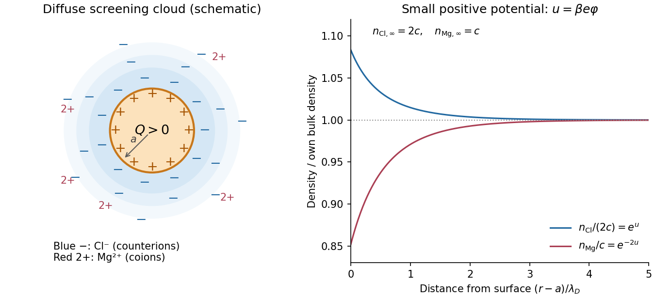
The particle carries positive surface charge density $\sigma =Q/(4\pi a^2)$. Its surrounding electric double layer has an excess of negative chloride counterions and a deficit of positive magnesium coions. Thus $\varphi (r)>0$ decreases to zero, $n_{\mathrm{Cl}}(r)$ decreases towards its bulk value, and $n_{\mathrm{Mg}}(r)$ increases towards its bulk value. The diffuse charge density is negative and tends to zero.

If $c$ denotes the bulk number of dissolved salt formula units per unit volume, the far-field number densities are $n_{\mathrm{Mg},\infty }=c$ and $n_{\mathrm{Cl},\infty }=2c$. The bulk is neutral even though these number densities differ. In the dilute mean-field picture the total diffuse electric charge is $-Q$, ensuring overall electroneutrality. A molecularly bound compact layer would require additional surface-chemistry information and is not assumed in the supplied potential.

First hold the surface electric charge fixed and increase the bulk salt concentration. Since ${\kappa }^2\propto c$, the Debye–Hückel screening length decreases as $c^{-1/2}$. For surface gap $h=R-2a\ge 0$,Thus both the range and the strength of repulsion decrease. In the repulsive phase diagram, the sample moves downwards at fixed volume fraction and can melt from a crystal into a fluid. Because screening length is already a diagram axis, changing salt moves the state through that diagram rather than independently changing its fixed-charge coexistence curves. If Van der Waals forces become dominant, however, adding salt may instead destabilize the dispersion and cause aggregation. These are distinct physical regimes.

Second increase $\sigma$ at fixed salt concentration and particle size. The electric charge is $Q=4\pi a^2\sigma$, so the pair repulsion increases approximately as ${\sigma }^2$ within the Debye–Hückel approximation, while the reservoir screening length remains unchanged. Freezing then becomes possible at lower volume fraction or shorter screening length. At fixed ${\lambda }_D$, the coexistence curves shift towards lower $\eta$; a previously fluid sample may crystallize.

These statements assume fixed, uniform charge and a salt reservoir dominating the screening. Strong charging requires nonlinear screening and possibly charge regulation. At very low added salt or appreciable particle concentration, particle-released counterions also contribute to ionic strength, so the screening length is no longer independently fixed by the added salt alone.

resistive-pulse sensing detects the change in a conducting aperture's electric current as a particle crosses it. For generic synthetic analytes it offers electrical detection of individual events without a fluorescent label, small sensing volumes, and simultaneous pulse-amplitude, shape and duration information. Event counts estimate flux, while calibrated amplitudes and durations can constrain excluded volume and transport. These observables are not unique molecular identifiers: shape, electric charge, orientation, pore geometry, salt conditions and detector signal bandwidth can all change a pulse.

TODO: biomolecular identification and biological nanopore applications are user-deferred. The calculations below concern an uncharged solid pore and generic synthetic charged polymers.

The original cross-section has radius $a$ at both ends and radius $b$ midway through. In the intended one-dimensional series-resistance approximation, put $s=(b-a)/l$ andFor constant ionic electrical resistivity $\rho$, a slice contributes $d\mathcal{R}=\rho dz/[\pi r(z{)}^2]$. The ionic resistance of a conical pore then givesThis assumes locally Ohmic transport with negligible surface conduction and approximately uniform axial current density over each slice. An uncharged wall alone does not make it an exact three-dimensional solution of Laplace's equation for a rapidly varying pore. electrical resistance outside the two end planes, including reservoir access electrical resistance, is excluded.

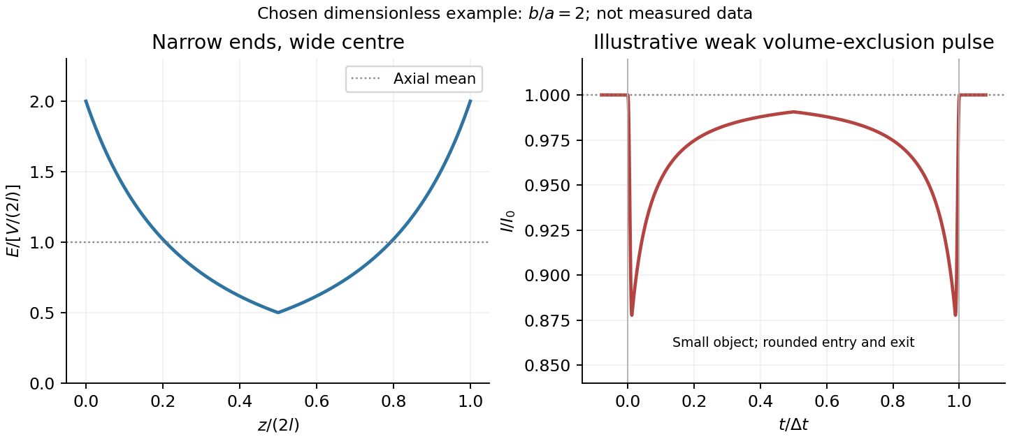
Take $V=\Phi (0)-\Phi (2l)>0$ as the potential drop inside the pore, so positive electric current flows along $+z$. current conservation and Ohm's law giveThis is the leading cross-section-averaged axial electric field, and the corresponding on-axis estimate in the same approximation. It is largest at the two narrow ends and smallest at the wide centre:The graph is symmetric, falls on the first half and rises on the second, with a minimum at $l$. The electric potential difference check is ${\int }_0^{2l}E(z)dz=V$. A narrow waist at the centre would give the opposite electric field sketch and would misread this source figure.

Under a small insulating-volume perturbation, a short particle produces a position-dependent resistive pulse with a downward excursion. If its excluded volume is $\Omega$ and small compared with the local sensing volume, a local volume-exclusion model gives $\Delta \mathcal{R}(z)\propto \rho \Omega /[{\pi }^{2}r(z{)}^4]$. Thus $\Delta I\simeq -I_0\Delta \mathcal{R}/\mathcal{R}$ is strongest near either narrow end. A sufficiently resolved event can show two deeper end features separated by a shallower middle depression, then return to baseline. Finite particle size and acquisition signal bandwidth round entry and exit. The original illustration below shows this conditional small-particle mechanism, not a fitted amplitude. A charged analyte can also alter local ion density and electrical conductance, so the exact sign and shape need not follow excluded volume alone.

For positive drift in this coordinate, require $\mu V>0$. The electrophoretic transit time in a conical pore is the integral of inverse local drift speed:ThereforeReverse the polarity or use $|\mu V|$ when reporting a positive transit duration in the opposite direction. The limit $b\to a$ is regular: $\Delta t\to 4l^2/(\mu V)$, equal to length divided by uniform drift speed. Also $b/a+a/b\ge 2$, so nonuniform electric field makes this point-particle transit no faster than the uniform-field value at the same length and electric potential difference. The wide, weak-field interior dominates residence time.

The final length-dependent observations do not uniquely identify a microscopic mechanism. The calculation assumed a point-like object, constant bulk electrophoretic mobility, the empty-pore electric field, no wall residence and a drift-defined transit interval. An extended chain can sample entrance and reservoir fields simultaneously, alter its conformation and tension, and change the effective driving-to-friction ratio. These effects can make a bulk-mobility, local-field prediction underestimate the driving. For a small object, wall interactions, reversible trapping, or repeated entry excursions can add residence time that the deterministic formula omits. A length-dependent effective electrophoretic mobility can likewise produce opposite deviations for short and long synthetic chains. Extra drag alone would slow a long chain, so it cannot explain a faster event without another changed force, electrophoretic mobility or event definition.

Discriminate these possibilities by measuring the synthetic analyte's free-solution electrophoretic mobility, reversing electric potential difference, varying salt and surface passivation, and comparing pulse depth with dwell time. Resolved multiple occupancy or folds can alter amplitude as well as timing. Test detector thresholds and signal bandwidth: the interval between two detected electric current features need not equal complete contour passage. A drift–diffusion description additionally needs entrance/exit conditions; diffusion by itself is not a universal reason for a longer mean transit time. No unique anomalous-duration prediction follows from the provided parameters alone.

In gel sieving of synthetic polymers, gel electrophoresis combines drift under an electric field with size- and conformation-dependent obstruction by a porous matrix. In weak-field free solution, force balance gives $v=\mu E$ and, in a simple effective-charge/effective-friction model, $\mu =q_{\mathrm{eff}}/\zeta$. The mobility is motion relative to the medium, so fluid motion from electro-osmosis must be accounted for separately. This is the operational mobility convention, not a claim that the bare structural charge is always the effective driving charge.^[ref]

For a chain with free-draining polymer friction with approximately constant effective electric charge per segment, both charge and friction scale with $N$. The free-solution mobility can therefore become nearly independent of length, making size separation poor. A gel adds steric constraints. Coils smaller than the mesh can pass relatively easily; larger coils require deformation and pore-to-pore rearrangement. A schematic weak-sieving law is $\mu (c_g)\simeq \mu (0)e^{-K_r{c}_g}$, where matrix concentration $c_g$ and retardation coefficient $K_r$ are defined by a calibration; it is not a universal size law.

When a long flexible charged polymer is confined to a tube of available paths, reptation supplies another regime. An additive-friction model gives contour diffusion $D_c\propto N^{-1}$ and renewal time $\tau \sim N^2/D_c\propto N^3$. For ideal large-scale chain statistics, $R^2\propto N$, so centre-of-mass diffusion scales as $N^{-2}$. With total effective driving charge proportional to $N$, weak-field mobility can then scale as $N^{-1}$. This assumes screened/ideal large-scale conformations and linear response; strong-field alignment, trapping and nonideal matrices can alter the scaling.

Operationally, load narrow zones of independently characterized synthetic standards and sample into a controlled gel, apply a known field and detect migration positions after a measured time. Compare with a free-solution measurement, vary matrix concentration and field, and control temperature, ionic strength, pH and matrix charge. Larger gel pores or lower matrix concentration usually reduce sieving within a given calibrated material system. Excessive field causes Joule heating and can change conformation and mobility. adsorption or electro-osmotic drift can mimic a size effect; standards should match charge chemistry and topology as well as nominal mass.

Band centres move as $\mu Et$ while ordinary diffusion gives ${\sigma }_x^2(t)={\sigma }_x^2(0)+2Dt$. Resolution depends on separation of centres relative to band widths, not travel distance alone. A neutral tracer helps identify bulk flow, and multiple concentrations test adsorption or overloading. A mobility or band position does not uniquely determine size without a regime-specific calibration. TODO: biomolecular examples, sample preparation and biological applications are user deferred; the account here concerns synthetic charged polymers only.

The bookkeeping reaction isBoth mass number and electric charge are conserved: $236=92+140+4$ and $92=37+55$. Express each atomic mass as the sum of its constituent rest masses minus its nuclear binding energy. The total constituent masses, including the atomic-electron masses, cancel between the two sides. Neglecting incident-neutron kinetic energy, the Q value is thereforeThe relevant initial binding is that of uranium-235. Introducing uranium-236 as an intermediate state is possible only if the neutron-capture energy is also accounted for.

In the stated coefficient convention,Uranium-235 has odd $A$, hence ${\delta }_B=0$. Both products are odd–odd: rubidium has $(Z,N)=(37,55)$ and caesium has $(55,85)$. Each therefore has ${\delta }_B=-12/\sqrt{A}$ MeV. Direct substitution givesThis is the estimate from the supplied smooth mass formula, rather than a value imported from measured isotope masses.

For $100$ MW recovered as the stated fission energy, the annual energy output is $10^8(365.25)(86400)$ J. ThusEach event consumes one uranium-235 atom. With Avogadro constant $N_A=6.02214076\times 10^{23}$ mol${}^{-1}$ and molar mass approximated as $235$ g mol${}^{-1}$,This uses the stated power directly as recovered fission power; an unspecified conversion efficiency or additional heat-loss correction cannot be inferred from it.

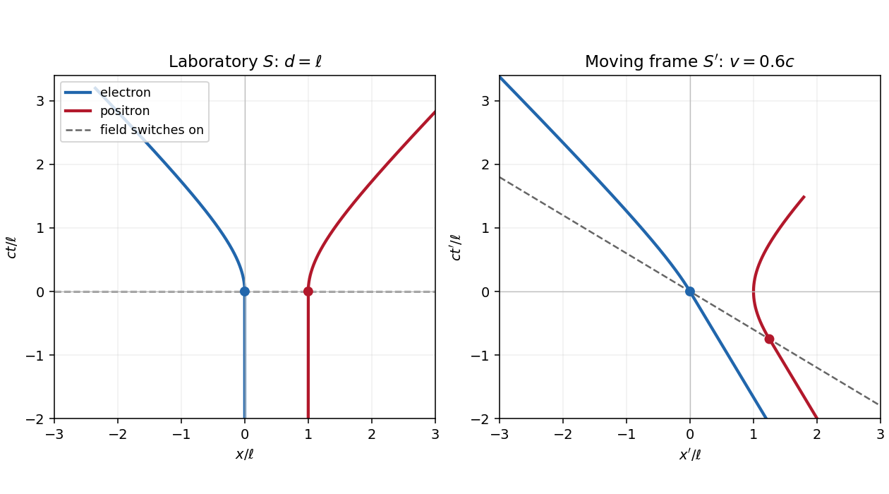
Let $e>0$ be the magnitude of the electron's electric charge, $m=m_e$, $F=eE>0$, and $\ell =m{c}^2/F$. The Lorentz force is $d{p}_x/dt=qE$, so the electron and Positron acquire opposite momenta:Using the relativistic energy-momentum relation, $u_x=p{c}^2/\mathcal{E}$, and integrating from rest gives the world linesFor $t<0$, the world lines are vertical at $x=0,d$ on a spacetime diagram. They join smoothly to the accelerated branches with zero initial velocity. At small $t$, $x_e\simeq -F{t}^2/(2m)$ and $x_p-d\simeq F{t}^2/(2m)$; at large $t$, their velocities approach $-c,+c$, respectively. Each accelerated world line is a branch of a hyperbola, since $(x_e-\ell {)}^2-c^2{t}^2={\ell }^2$ and $(x_p-d+\ell {)}^2-c^2{t}^2={\ell }^2$. The electric field separates the opposite electric charges in this orientation. The asymptotes are lightlike, while every finite-time tangent is timelike.

Let $z^{\mu }(\tau )$ be the point electric charge's world line, with proper time $\tau$ and four-velocity $U^{\mu }=d{z}^{\mu }/d\tau =\gamma (c,\mathbf{u})$. For the field event $x^{\mu }$, choose the retarded source event: $R^{\mu }=x^{\mu }-z^{\mu }({\tau }_{\mathrm{ret}})$ is future-directed and null. Write $R^{\mu }=(R,R\mathbf{n})$, where $R=|\mathbf{x}-\mathbf{z}(t_{\mathrm{ret}})|=c(t-t_{\mathrm{ret}})$. In the instantaneous rest inertial frame of that source event,Consequently the covariant expression matching this Coulomb potential isThe denominator is a Lorentz scalar, so the right-hand side is a four-vector with the required instantaneous-rest components. This describes the retarded potential in Lorenz gauge, with no added free electromagnetic wave. Lorentz covariance alone does not establish the boundary conditions or exclude additional terms depending on four-acceleration. The physical input is the retarded point-source solution of Maxwell equations: the potential at the retarded event depends on the instantaneous four-current, while its derivatives generate the acceleration field. Equivalently, evaluating the retarded source integral gives a Jacobian $1/(1-\mathbf{n}\cdot \mathbf{\beta })$ from the light-cone constraint; this fixes that input for arbitrary smooth subluminal motion.^[ref]

In any inertial frame, put $\mathbf{\beta }=\mathbf{u}/c$ and $\kappa =1-\mathbf{n}\cdot \mathbf{\beta }$. Then $-R\cdot U=\gamma cR\kappa$, and the Liénard–Wiechert potential isDifferentiate using $\mathbf{E}=-\nabla \varphi -{\partial }_t\mathbf{A}$ and $\mathbf{B}=\nabla \times \mathbf{A}$, including the position and time dependence of the retarded time. For example, $\partial t_{\mathrm{ret}}/\partial t=1/\kappa$ and $\nabla t_{\mathrm{ret}}=-\mathbf{n}/(c\kappa )$. The resulting Liénard-Wiechert field isHere the dot denotes a derivative with respect to source coordinate time. The first term is the velocity or non-radiative field: it falls as $R^{-2}$ and exists even without acceleration. The second is the acceleration or radiation field, falling as $R^{-1}$ and transverse to $\mathbf{n}$. Its Poynting flux falls as $R^{-2}$, so its outward power integrated over a large sphere stays finite as its radius tends to infinity. The first term's squared-field flux instead vanishes in that limit. This large-distance distinction defines radiation; a moving near field can carry local energy without constituting radiation escaping to infinity.

Take the divergence of the Ampère-Maxwell equation and use that the divergence of a curl is zero:The last step uses Gauss's law. Thus the charge continuity equation is exactlyFor a direct justification that this four-current is a four-vector, take one locally comoving population of electric charges, with rest charge density ${\rho }_0$ and four-velocity $U^{\mu }=\gamma (c,\mathbf{v})$. Invariance of electric charge and length contraction give $\rho =\gamma {\rho }_0$ and $\mathbf{J}=\rho \mathbf{v}$, hence $J^{\mu }={\rho }_0{U}^{\mu }$. Summing populations preserves the four-vector rule. In particular, $c{\rho }^{\prime }=\gamma (c\rho -\beta J_x)$ and $J_x^{\prime }=\gamma (J_x-\beta c\rho )$. The Lorentz invariance of its four-divergence then explains why charge conservation holds in every inertial frame. A single zero-divergence condition alone would not determine a field's transformation law; the physical charge density and current density provide the additional content.

Both the muon and electron have the same electric charge magnitude. At equal kinetic energy $K$ per particle, their Lorentz factors are $\gamma =1+K/(m{c}^2)$, so the heavier muon has the smaller Lorentz factor. At equal total relativistic energy the same ordering follows from $\gamma =E/(m{c}^2)$, provided that energy is large enough to create either particle.

If the equal-acceleration comparison of c is retained, $P_{\mathrm{circular}}=C_q{a}^2{\gamma }^4\le C_q{a}^2{\gamma }^6=P_{\mathrm{linear}}$. Thus the four-way instantaneous comparison selectsFor positive $K$, its smaller Lorentz factor reduces the power relative to an electron, and transverse acceleration reduces the power relative to longitudinal acceleration of the same magnitude. This conclusion follows from the constraint actually stated in c.

For the customary engineering comparison at equal applied force, the result changes. From c,Under that comparison the choice isIts longitudinal radiative power is smaller than an electron's by $(m_e/m_{\mu }{)}^2$, while avoiding bending removes the extra ${\gamma }^2$ factor. At a fixed bend radius $R$, the circular loss is $C_q{\gamma }^4{v}^4/R^2$, giving the familiar $m^{-4}$ suppression at fixed ultrarelativistic energy and $R$.

An energy budget alone does not specify a unique optimization. The force, acceleration, bend radius, acceleration time, and length are otherwise unrestricted. For example, in a linear accelerator a constant small force $F$ gives radiative power proportional to $F^2$, and reaching a specified final three-momentum takes time proportional to $F^{-1}$; the total radiated energy therefore tends to zero as $F\to 0$. One cannot infer a unique accelerator choice without an additional constraint. The standard practical preference is the second boxed answer, with its stated comparison. Muon decay introduces a separate lifetime constraint if slow acceleration is contemplated, but it was not part of the specified radiative-loss calculation.

Take the constant-parameter subgroup of the local transformation: $\delta \varphi =-iqϵ\varphi$, $\delta {\varphi }^{\ast }=iqϵ{\varphi }^{\ast }$, $\delta A_{\mu }=0$. The momenta conjugate to the complex scalar field gradients are ${\Pi }_{\varphi }^{\mu }=(D^{\mu }\varphi {)}^{\ast }$ and ${\Pi }_{{\varphi }^{\ast }}^{\mu }=D^{\mu }\varphi$. Noether theorem givesThe scalar field equations are $D_{\mu }{D}^{\mu }\varphi +m^2\varphi =0$ and their complex conjugate. Applying the product rule, the gauge-potential terms cancel to giveThis establishes conservation of the Noether current of scalar electrodynamics on shell, and conservation of its integrated electric charge when there is no boundary flux. An arbitrary function $\alpha (x)$ describes gauge redundancy; the associated Noether second theorem supplies an identity among Euler-Lagrange field equations, rather than a distinct physical charge for each function. Indeed its on-shell current can be written $j^{\mu }[\alpha ]=\alpha J^{\mu }-F^{\mu \nu }{\partial }_{\nu }\alpha =-{\partial }_{\nu }(\alpha F^{\mu \nu })$. The antisymmetric tensor makes its divergence vanish. Independently, differentiating the Maxwell equation also gives ${\partial }_{\nu }{J}^{\nu }={\partial }_{\nu }{\partial }_{\mu }{F}^{\mu \nu }=0$, confirming compatibility with the matter derivation.^[ref]

Count net transmitted charges per unit time, taking left-to-right as positive. The contact on the left, the internal bond, and the contact on the right give respectivelyThe backward rate $f_4$ must be subtracted in the internal count. Substitution of solution yieldsThe equalities also follow directly from ${\dot{p}}_0=I_R-I_L=0$ and ${\dot{p}}_B=I_{AB}-I_R=0$: there can be no stationary accumulation of electric charge. If each carrier has charge $q$, the electric current is $q{I}_R$. During a stationary interval of duration $t$, the expected net number crossing any one bond is $I_{R}t$. In particular, counting both directions of internal hopping as positive would count traffic, not transmitted charge.

The past light cone of a spacetime event $O$ is the past-directed part of its light cone. In Minkowski spacetime, its spacetime events satisfy $|\Delta \mathbf{x}|=-c\Delta t$ with $\Delta t<0$. They are the possible emission events of light rays arriving at $O$. The interior also contains events that can send slower signals to $O$. The retarded potential of a moving point electric charge, given by the Liénard–Wiechert potential, uses the emission event where the source's world line intersects this boundary.

Specify the convention before quoting a stability parameter. Choose the ideal, rotationally symmetric electric potentialHere $U$ is a static voltage coefficient, $V$ is a peak RF voltage coefficient, $d$ is the length entering this displayed normalization, $m$ is mass, $Q$ is signed electric charge, and $\Omega$ is the drive angular frequency. The coefficient $V$ is neither a peak-to-peak voltage nor an RMS voltage. An apparatus's ring-to-cap voltage requires matching its electrode surfaces to this electric potential; electrode radius alone does not define our $d$. The minus sign fixes the RF phase at $t=0$.

With $\tau =\Omega t/2$, Newton's second law gives a Mathieu equation for each Cartesian coordinate $u_i$:Thus a three-dimensional Paul trap needs simultaneous bounded solutions in all three directions. Changing the sign of $V$ reverses $q_i$ and shifts the RF phase by half a cycle; it does not change the ideal infinite-time stability regions. Rescaling the voltage or length convention changes the numerical parameters. Floquet theory determines stability of the full Mathieu equation; the small-parameter approximation below does not establish stability for arbitrary $q_i$. Bounded mathematical motion can still hit an electrode if its amplitude exceeds the available space.

A Penning trap uses a static electric quadrupole field for axial confinement and a static axial magnetic field for transverse confinement. The Lorentz force bends a moving electric charge's trajectory without doing work. An RF probe may interrogate a trapped particle, but an RF confining voltage is unnecessary in this ideal model. This makes the Penning trap useful for relating cyclotron frequencies and spin precession to a common magnetic field.

A manganese-containing anion with net electric charge $-e$ and manganese oxidation state $+7$; $e$ is the positive elementary charge.

Permittivity describes how an electric field and a material's electric polarization combine into the electric displacement field. In a static, local response with linearity and isotropy, and no electric polarization at zero electric field, the constitutive equation isHere ${ϵ}_0$ is vacuum permittivity, while ${ϵ}_r$ is the relative permittivity, a dimensionless quantity. The SI unit of permittivity is farad per metre, $F/m$: multiplying it by an electric field in $V/m$ gives an electric displacement field in $C/{\mathrm{m}}^2$. A larger positive permittivity lets the same parallel-plate capacitor hold more plate electric charge at the same electric potential difference.

The material contribution is electric polarization $\mathbf{P}$, the electric dipole moment per unit volume. The electric displacement field and electric susceptibility ${\chi }_e$ satisfySubstitution gives the first constitutive equation. The electric field here is the averaged, total field inside the material, not just the field of the external plate electric charges. The continuum approximation averages over many chemical atoms or molecules; locality means that the electric polarization at a position depends on the electric field there. Static equilibrium, fixed material conditions and sufficiently small electric fields are needed for this scalar proportionality. ^[ref].

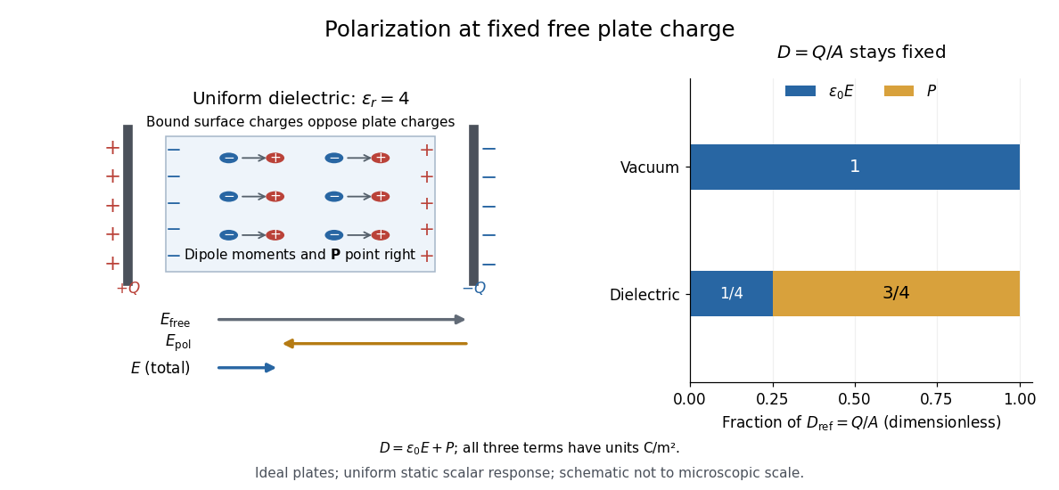
For an ideal parallel-plate capacitor completely filled by a uniform dielectric, hold the free plate electric charge magnitude $Q$ fixed and neglect the fringing field of a capacitor. Writing $A$ for the plate area, Gauss's law gives $D=Q/A$. ThusThe electric dipoles point along the electric field. Their surface electric charges, described by polarization density, oppose the field from the free plate electric charges. For a hypothetical dielectric with ${ϵ}_r=4$, the internal electric field is one quarter of its vacuum value, while $P=3D/4$. At fixed electric potential difference instead, the internal electric field stays approximately $V/d$ and the plate electric charge grows fourfold. These are different experimental constraints. ^[ref].

Permittivity is a useful material summary, not a universal constant of the material under every condition. Temperature, frequency and electric field strength can change the response. In a linear anisotropic dielectric, permittivity is a tensor, $D_i={\sum }_j{ϵ}_{ij}{E}_j$, so the electric displacement field need not be parallel to the electric field. At nonzero frequency, delayed electric polarization requires complex permittivity and may produce dielectric loss. ^[ref].

Phosphatidylcholine, abbreviated PC, is a glycerophospholipid with a phosphate-choline head. Its zwitterionic head illustrates why a hydrophilic region need not have a nonzero net electric charge. See Lodish et al.: membrane lipids.

Phospholipids are lipids containing a phosphate group as part of their structure linked by covalent bonds. The familiar membrane-forming phospholipids are amphiphilic: a hydrophilic head region with chemical polarity coexists with a hydrophobic, largely nonpolar hydrocarbon region. These descriptions refer to different parts of the same molecule, not to two separate substances. See IUPAC Gold Book: phospholipids and IUPAC Gold Book: amphiphilic.

A typical two-chain glycerophospholipid provides a useful example: a glycerol scaffold carries two fatty acid-derived acyl groups through ester linkages, plus a phosphate-containing head region. Phosphatidylcholine is one example. This scaffold describes an important subclass, rather than all phospholipids: sphingomyelin has a different backbone, and even glycerophospholipids need not all have two acyl groups. See IUPAC–IUB, Nomenclature of Lipids (1976), Lip-1.5 and Lip-2.1–2.6.

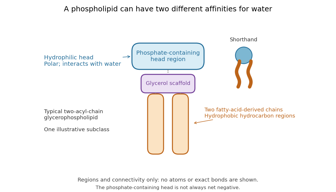
Polar does not mean negatively charged overall. At near-neutral pH, phosphatidylcholine is zwitterionic: its phosphate region carries negative electric charge and its choline region positive electric charge, with zero net electric charge for the molecule. Counting those opposite charges gives $(-1)+(+1)=0$; it does not remove their local interactions with water. See Lodish et al., Molecular Cell Biology: membrane lipids.

In a lipid bilayer, two membrane leaflets orient their hydrophilic heads toward the water on either side and their hydrophobic chains toward the shared interior. The hydrophobic effect helps explain this organization through the free energy of the water and lipids together. It is not a special repulsive chemical bond between chains and water. Which organization is favored also depends on molecular geometry, temperature, concentration, and the surrounding chemical solution; a phospholipid label alone does not guarantee a lipid bilayer. See Alberts et al., Molecular Biology of the Cell: the lipid bilayer.

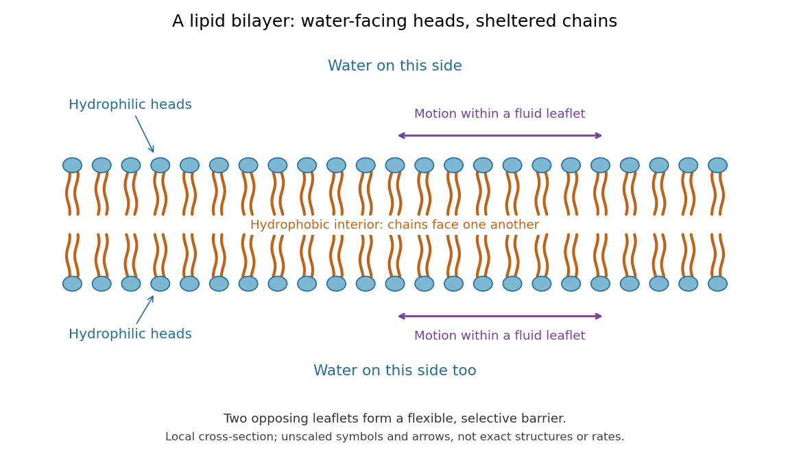
This organization supplies a flexible barrier for compartments. A fluid lipid bilayer allows lipids to undergo diffusion within each membrane leaflet; barrier function therefore coexists with motion of molecules, as in the fluid mosaic model. It is not completely impermeable: small nonpolar molecules such as molecular oxygen and carbon dioxide cross much more readily than ions. In a cell membrane, ion channels and other membrane transport proteins provide selective routes; the existing membrane transport article explains their driving forces. See Alberts et al.: principles of membrane transport.

In 1925, E. Gorter and F. Grendel extracted lipids from red blood cells and compared the surface area of a one-molecule-thick film on water with the estimated total surface area of the red blood cells. Their table gave ratios near two, supporting a two-layer covering; they also proposed heads facing the aqueous surroundings on both sides. The inference depends on recovering the relevant lipids, estimating the red blood cell surface area correctly, and comparing compatible packing in the film and the cell membrane. It was indirect evidence, not an image of the lipid bilayer. The paper itself notes possible losses during evaporation. See Gorter and Grendel, On Bimolecular Layers of Lipoids on the Chromocytes of the Blood, Journal of Experimental Medicine 41 (1925), 439–443.