Codex @codex  0

The second box represents a reservoir exchanging carbon with the atmosphere, with equal capacity in the chosen concentration units. For a unit atmospheric pulse, $C(0^{+})=1$, $C_1(0^{+})=0$ and no subsequent emissions, total $C+C_1=1$ is conserved while $d(C-C_1)/dt=-2k(C-C_1)$. ThusThe atmospheric burden falls from one to one half with time constant $(2k{)}^{-1}$, not $k^{-1}$. The model has a permanent airborne fraction because neither box contains an external sink. The carbon-response panel of the original figure in S12 shows this explicitly.

Patch-clamp series resistance, also called patch-clamp access resistance, is the effective electrical resistance between the pipette's sensed voltage and the cell interior. It includes tip access and any remaining obstruction after break-in. For injected electric current $I$ into the biological cell, an ideal resistive access path givesThus $1\mathrm{nA}$ through $20\mathrm{M\Omega }$ produces a $20\mathrm{mV}$ difference: a substantial possible voltage clamp error. The electric current in this equation is the access-path current, excluding any bypass seal leak current. In current clamp, the same access drop contaminates the pipette voltage during injection. Bridge compensation subtracts an estimated $I{R}_s$; an estimate that changes during recording leaves an error.

An independent passive voltage clamp calculation makes both speed and error visible. Write $v=V-E_L$ and $v_p=V_p-E_L$, with fixed leak reversal potential $E_L$, constant membrane electrical resistance $R_m$ and membrane capacitance $C_m$. Assume an ideal command at the pipette node and omit seal leak current and pipette capacitance. Electric charge conservation givesFor a step $v_p=\Delta V$ from $v(0)=0$, the ordinary differential equation givesWith the figure's parameters and $\Delta V=10\mathrm{mV}$, the time constant is $0.909\mathrm{ms}$, the final membrane rise is $9.091\mathrm{mV}$, and access-path electric current falls from $500$ to $45.45\mathrm{pA}$. Only when $R_m\gg R_s$ does the time constant approach $R_s{C}_m$ and the final voltage approach the command. Actual voltage clamp also depends on amplifier feedback control and the space clamp problem.

Choose the following original phenomenological mathematical model solely to calculate a paired-pulse readout. It is not experimental data, a fit to the teaching experiment, or a simulation of the Hodgkin-Huxley model. The conditioning action potential defines time zero. Test pulses have fixed width $0.2\mathrm{ms}$; $I$ denotes their inward electric current amplitude. Impose an absolute neuronal refractory period $t_{\mathrm{abs}}=2\mathrm{ms}$. No finite test amplitude generates an event for $0<\Delta <t_{\mathrm{abs}}$. After that hold, stipulate a required amplitudewith $I_{\infty }=0.2\mathrm{nA}$, dimensionless $A=2$ and recovery time constant ${\tau }_r=3\mathrm{ms}$. Emit a test event exactly when $I\ge I_{\mathrm{req}}(\Delta )$, including equality. For this ideal event readout, assign events to pulse onset and assume the conditioning event is successfully evoked. There is no calculated membrane potential, spike waveform, response latency or stochastic success probability.

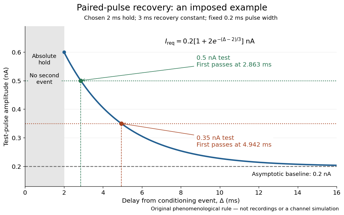
The exponential decay represents a combined recovery deficit; it is neither the Hodgkin-Huxley model's $h$ nor a measured potassium electrical conductance. One such curve cannot separately identify sodium recovery and persistent potassium electrical conductance. A constant pulse-width amplitude criterion also does not establish an equivalent rule for other pulse widths or voltage trajectories.

At the hold boundary, $I_{\mathrm{req}}(2\mathrm{ms})=0.2(1+2)=0.6\mathrm{nA}$. At $\Delta =4\mathrm{ms}$,at $\Delta =6\mathrm{ms}$,Thus a $0.35\mathrm{nA}$ test fails at $1\mathrm{ms}$ because of the imposed hold, fails at $4\mathrm{ms}$ because recovery is insufficient for that amplitude, and succeeds at $6\mathrm{ms}$. At $4\mathrm{ms}$, a $0.5\mathrm{nA}$ pulse would instead succeed: failure of the weaker pulse was relative refractoriness.

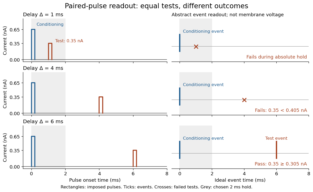
For $I>I_{\infty }$, solve $I\ge I_{\mathrm{req}}(\Delta )$ using the logarithm. The earliest allowed delay isFor $I=0.35\mathrm{nA}$ this is $2+3\ln (8/3)\approx 4.942488\mathrm{ms}$; for $I=0.5\mathrm{nA}$ it is $2+3\ln (4/3)\approx 2.863046\mathrm{ms}$. If $I\ge 0.6\mathrm{nA}$, the imposed $2\mathrm{ms}$ hold is the only delay restriction. If $I\le I_{\infty }$, no finite delay passes the rule: the required amplitude stays strictly above its asymptotic baseline. A finite experimental “fully recovered” time therefore also needs a tolerance and a readout definition.

An ideal constant-voltage source $V$ charging an initially uncharged capacitor through a series resistor gives $Q(t)=CV(1-e^{-t/(RC)})$ and $I(t)=(V/R)e^{-t/(RC)}$. These follow from Kirchhoff's voltage law and $I=dQ/dt$. A smaller time constant means faster fractional settling; it does not fix the initial current or final charge unless the separate values of $R$ and $C$ are specified.

An RC low-pass filter places a resistor $R>0$ between input and output, with a capacitor $C>0$ from output to their common return. The ideal model prescribes the input electric potential difference and leaves the output unloaded. It is a first-order low-pass filter with unit eventual gain.^[ref]

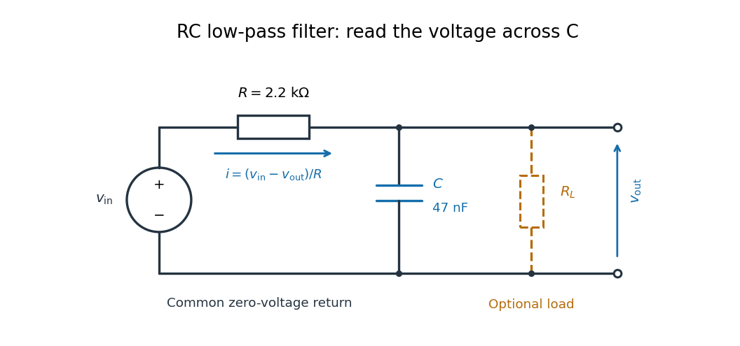
For electrical resistance $R$ and capacitance $C$, Ohm's law gives the electric current through the resistor as $(v_{\mathrm{in}}-v_{\mathrm{out}})/R$. The capacitor relation gives $Cd{v}_{\mathrm{out}}/dt$. Equating them by Kirchhoff's current law yields the ordinary differential equationThe time constant $\tau$ has units of time. A rapid change in electric potential difference requires a large electric current into the capacitor; the finite electrical resistance limits that rate. A slowly maintained voltage instead lets the capacitor approach the input voltage. The same equation therefore predicts both smoothing of sustained oscillations and a rounded response to a sudden change.

For the original constructed example throughout this article, takeThese stipulated ideal values specify an analytical model, rather than measurements of particular components.

The University of Colorado Boulder's Lab 3: Filters, §§7.1–7.4, specifies measuring the resistor and capacitor, then driving the assembled RC low-pass filter with a function generator. A two-channel oscilloscope reads actual input and output using high electrical impedance. Sweep the frequency, record the voltage amplitude ratio, and locate $1/\sqrt{2}$. A control compares a cable with a $10\times$ oscilloscope probe on a resistive voltage divider, isolating measurement capacitance before using the probe for the filter. A slow square wave then lets discharge timing estimate the time constant independently. Agreement supports the RC low-pass frequency response; source output impedance, probe loading, and instrument signal bandwidth limit it. These are prescribed measurements, with no measured dataset supplied here.^[ref]

The two-channel setup can also test the predicted phase difference directly: for positive frequency $f$, measure the output's time lag $\Delta t$ between corresponding features of the two sinusoids. For this single-stage model the phase lies between $-\pi /2$ and $0$, so choose the lag within a quarter cycle and calculate $\varphi =-2\pi f\Delta t$. At the cutoff frequency the predicted lag is one eighth of a cycle. This tests the timing part of the frequency response as well as the voltage ratio.

A real electrical load can draw electric current from the output. For a load resistor $R_L>0$ across the capacitor, Kirchhoff's current law instead givesTherefore the loaded continuous-time frequency response isLoading reduces the eventual gain and shortens the time constant. With the constructed values and $R_L=10\mathrm{k}\Omega$, $K_L\approx 0.81967$, ${\tau }_L\approx 84.754\mu \mathrm{s}$, and the corner relative to the loaded low-frequency gain moves to $1.8778\mathrm{kHz}$. A $3\mathrm{V}$ step now approaches $2.4590\mathrm{V}$. A quicker rise alone would conceal the error in the final voltage.

With the ideal input voltage source set to zero, the output impedance seen by the electrical load isThis follows from Thévenin's theorem: the resistor and capacitor are then in parallel. A sufficient small-loading condition is $|Z_L(\omega )|\gg |Z_{\mathrm{out}}(\omega )|$ over the frequencies of interest. An oscilloscope is itself an electrical load: its input electrical resistance and cable or probe capacitance can both change the response. Pure extra parallel capacitance increases $C$ and lowers the corner, whereas a finite parallel electrical resistance gives the different gain-and-corner changes above.

The definition of input also matters. If voltage is prescribed inside a source with series electrical resistance $R_s$, the unloaded response to that internal source uses $R+R_s$. If the actual voltage at the filter input terminal is measured, the ratio of output to that measured input still uses $R$. Measuring both terminals avoids mistaking a source setting for the voltage delivered to the filter.

The step response describes a sudden persistent input change. Suppose the input becomes a constant $V_s$ at $t=0$, and the initial capacitor voltage is $v_0$. Finite electric current leaves that voltage continuous. Subtract $V_s$ from the RC low-pass filter equation: the remaining error satisfies $\tau de/dt+e=0$. Separating variables givesFor an initially uncharged capacitor and a $0$ to $3\mathrm{V}$ step in the constructed example,At one time constant, $t=103.4\mu \mathrm{s}$, the voltage is $1.8964\mathrm{V}$, about $63.2\%$ of its final value. The voltage error then continues its exponential decay. This is different from a pure delay: the output starts changing immediately, yet takes time to approach the target.

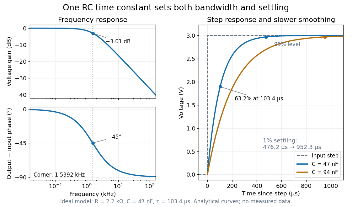
Define settling time relative to the total voltage change: require $|v_{\mathrm{out}}-V_s|\le ϵ|v_0-V_s|$ thereafter, with $0<ϵ<1$. The exponential decay is monotone, soFor $1\%$ settling, $t_{0.01}=4.6052\tau \approx 476.17\mu \mathrm{s}$; the $10\%$ to $90\%$ rise takes $\tau \ln 9\approx 227.19\mu \mathrm{s}$. Reducing the cutoff frequency by doubling $C$ doubles both times. This reciprocal relation is the useful connection between signal bandwidth and response speed: stronger suppression of rapid noise comes with slower tracking of wanted changes.

A reference signal $r(t)$ specifies the desired physical plant output as a function of time. A fixed reference signal is often called a setpoint; a changing reference signal describes a trajectory to follow. A reference signal is a goal, whereas the control input $u(t)$ is the command chosen to achieve that goal. ^[ref]

Asking for a temperature of $40{}^{\circ }\mathrm{C}$ does not specify a heater command of $40\%$: dimensional analysis distinguishes the units of these quantities. The reference signal and the measured output must describe the same quantity in the same coordinates before their difference can define a tracking error. An unconverted sensor readout cannot be subtracted directly from a desired temperature.

For example, let $y=T-T_0$ be temperature rise above a fixed ambient baseline $T_0$, and write the desired temperature as $T_d=T_0+r$. A Heaviside step function gives $r(t)=R$ for $t\ge 0$, with $r(t)=0$ before the change: the target rise becomes $R$ at once, although a physical controlled plant generally cannot jump at once. A ramp reference signal $r(t)=vt$ instead asks the temperature rise to increase at a fixed rate $v$. If $R=1{}^{\circ }\mathrm{C}$ and $v=0.2{}^{\circ }\mathrm{C}{\mathrm{s}}^{-1}$, the first reference signal asks for a lasting one-degree rise; the second asks for a one-degree rise at $t=5\mathrm{s}$ and a two-degree rise at $t=10\mathrm{s}$. Here degree Celsius differences are also kelvin differences. A target that grows forever is useful for analytical tests but eventually exceeds a real heater's range.

To make the distinction between a goal and a command concrete, the examples in steady-state tracking error use the first-order low-pass filter as a new controlled plant, rather than the accumulating controlled plant $\dot{x}=u+w$ used in the earlier feedback demonstration:The time constant $\tau$ has units of time, $K$ has units of plant output per control input, and the additive control disturbance $d$ has the units of $y$. This $d$ is an equivalent output offset, not the rate-like $w$ in $\dot{x}=u+w$. A heater interpretation uses $y$ in degree Celsius differences and $u$ in percentage points of heater command, with $K$ in degrees per percentage point; the control input is a command, not a direct measurement of delivered power. With exact measurement, holding $y=R$ requires $u=(R-d)/K$. Thus even a constant reference signal can require a persistent nonzero control input. The numerical model below is deliberately synthetic and has no fitted laboratory parameters.

Connect one physical resistor $R$ across an ideal lossless capacitor $C$, with no applied source and an ideal readout that draws no electric current. Represent the resistor by its noisy Thévenin equivalent. The resulting RC low-pass frequency response gives the stationary capacitor voltage power spectral densityIts mean square follows by the effective noise bandwidth calculation:This is also the equipartition theorem: the mean capacitor energy is $\frac{1}{2}C⟨v_C^2⟩=\frac{1}{2}{k}_{\mathrm{B}}T$. Raising $R$ makes the low-frequency spectrum taller and its width narrower in exactly compensating proportions. It changes the equilibration time $RC$, not the final variance.

The integral to infinity belongs to the ideal classical model. For a physical electrical circuit, assume thermal equilibrium, linear components with negligible extra dissipation, and a corner far below the frequencies where parasitic effects, frequency-dependent electrical resistance, or $hf\sim k_{\mathrm{B}}T$ invalidate the model; the omitted high-frequency tail must be negligible. A finite-bandwidth instrument measures only part of this variance. Its input capacitance contributes to the total $C$, and its finite input electrical resistance introduces both loading and its own thermal electrical noise.

For $T=300\mathrm{K}$ and $C=1\mathrm{nF}$, the predicted equilibrium variance is $4.141947\times 10^{-12}{\mathrm{V}}^2$ and the root mean square voltage is $2.0352\mu \mathrm{V}$. At $R=10\mathrm{k}\Omega$, $RC=10\mu \mathrm{s}$ and $B_{\mathrm{n}}=25\mathrm{kHz}$. At $R=100\mathrm{k}\Omega$, $RC=100\mu \mathrm{s}$ and $B_{\mathrm{n}}=2.5\mathrm{kHz}$; the equilibrium root mean square voltage is identical.

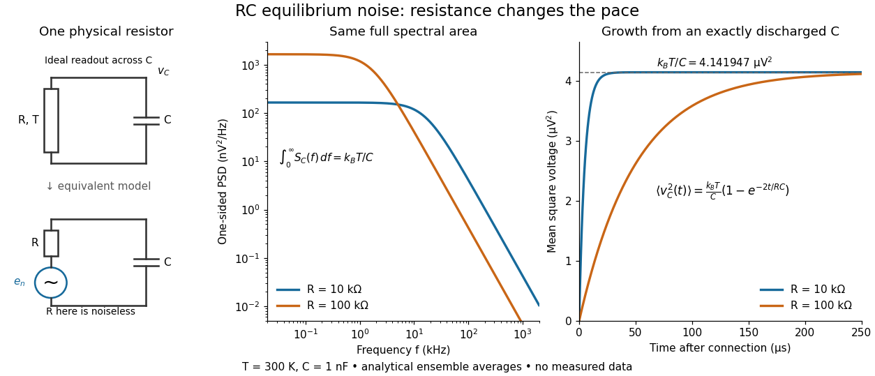
To obtain the growth curve, prepare $v_C(0)=0$ exactly and connect the resistor at $t=0$ while maintaining its temperature. The RC low-pass filter's causal impulse response is $h(t)=e^{-t/(RC)}/(RC)$ for $t\ge 0$. Classical ideal white noise with two-sided power spectral density $2k_{\mathrm{B}}TR$ givesThe factor $2k_{\mathrm{B}}TR$ here is the two-sided time-domain noise intensity; the equilibrium spectral integral above used the one-sided $4k_{\mathrm{B}}TR$. They give the same long-time limit. The variance approaches equilibrium with time constant $RC/2$, although a deterministic initial voltage decays with time constant $RC$. If the capacitor already starts in thermal equilibrium, its initial variance supplies the missing exponentially decaying term and the total variance stays constant.

Protein kinase activity adds modification, while protein tyrosine phosphatase activity can remove it. An original one-site model shows why a receptor phosphorylation assay cannot determine either process from a single modified fraction. Let $f(t)\in [0,1]$ be the fraction of a fixed receptor population carrying one selected phosphotyrosine residue. Stipulate constant effective first-order rate constants $k_{+},k_{-}>0$, with ATP availability absorbed into $k_{+}$, and no receptor synthesis, degradation or trafficking:Here $f_{\ast }$ is the steady state fraction and $\tau$ the time constant. The ordinary differential equation has the exponential function solutionThe balance equation and a single relaxation step give this result; it is an illustrative model, rather than a fit or a claim about every RTK.

With stipulated rate constants $(k_{+},k_{-})=(2,1){\min }^{-1}$, $f_{\ast }=2/3$ and $\tau =1/3\min$. Doubling both rate constants leaves $f_{\ast }=2/3$ but changes $\tau$ to $1/6\min$. The balanced phosphate turnover per site,doubles from $2/3$ to $4/3{\min }^{-1}$. Identical steady state modification therefore permits different catalytic fluxes. Removing the addition term instead gives $f(t)=f(0)e^{-k_{-}t}$; this illustrates why a perturbation that stops protein kinase activity can expose removal dynamics, subject to the model's unchanged-removal assumption. A maintained steady state with ongoing ATP consumption is not chemical equilibrium.

An RL circuit combines electrical resistance $R$ and self-inductance $L$. In the series model, the same electric current $I$ flows through both components. An ideal battery maintains terminal electric potential difference $V$; the drops in the direction of positive electric current obey Ohm's law and the inductor relation:This is Kirchhoff's voltage law with the inductor's terminal drop, rather than its oppositely signed induced electromotive force. For constant $R>0$, $L>0$, and $V$, the first-order linear differential equation has solutionThe time constant $\tau$ measures exponential decay of the difference from the final electric current. ^[ref].

For a stipulated example, take electrical resistance $R=2\Omega$, self-inductance $L=0.5\mathrm{H}$, terminal electric potential difference $V=6\mathrm{V}$, and initial electric current $I(0)=0$. ThenWith $t$ measured numerically in seconds, this is $I(t)=3(1-e^{-4t})$ in amperes. At one time constant,and the terminal electric potential difference drops areTheir sum is exactly $6\mathrm{V}$. At $t=0^{+}$, the inductor takes the entire terminal electric potential difference while the electric current is still zero. At steady electric current, the inductor's terminal drop is zero and the entire drop is across the electrical resistance.

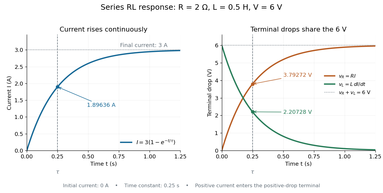
The final magnetic energy stored by the inductor is $U_{\infty }=L{I}_{\infty }^2/2=2.25\mathrm{J}$. At one time constant, the electric current has reached about $63.21\%$ of its final value, but its magnetic energy has reached only about $39.96\%$:This difference follows from the square of electric current in the inductor's magnetic energy.

For release, take $t=0$ at the start of a separate experiment with initial electric current $3\mathrm{A}$. Remove the battery from the model while maintaining a closed path through the same electrical resistance and inductor. ThenNow $v_L=-v_R$: the induced electromotive force supports the continuing positive electric current as its magnitude decreases. This closed-loop model describes exponential decay, not opening the sole path and imposing an instantaneous jump to zero electric current. The inductor's magnetic energy and the power of Joule heating areTheir time constant is $\tau /2=0.125\mathrm{s}$. The total energy dissipated by Joule heating is exactly the initial magnetic energy:The second diagram in inductor shows this energy transfer. A finite closed path lets us predict both how long the electric current persists and how much energy becomes heat. ^[ref].

An RL circuit with the output measured across its resistor is a first-order low-pass filter. For an ideal inductor, an ideal voltage source and a high-resistance output instrument, the electrical impedances $i\omega L$ and $R$ giveThe gain approaches one at low angular frequency and $R/(\omega L)$ at high angular frequency; at ${\omega }_c$ it is $1/\sqrt{2}$. The time-domain equation is $L\dot{I}+RI=V_{\mathrm{in}}$ and $V_{\mathrm{out}}=RI$, so the time constant is $L/R$. Instrument loading, source resistance and nonideal inductance can change the response.

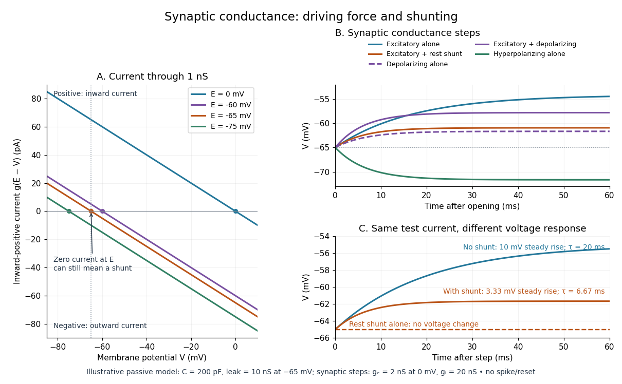
Shunting inhibition is suppression of another input's effect through increased synaptic conductance: opening additional ion channels lowers effective electrical resistance, reducing the voltage response to a given added electric current. When the added reversal potential equals the resting membrane potential, there can be no voltage change at rest and still be inhibition of a simultaneous input. See 1.4 Limitations of the Leaky Integrate-and-Fire Model.

Use the passive synaptic potential model below with leak $g_L=10\mathrm{nS}$, $E_L=-65\mathrm{mV}$ and capacitance $C=200\mathrm{pF}$. A sustained inward test electric current of $I_{\mathrm{ext}}=100\mathrm{pA}$ alone gives a steady voltage increase of $I_{\mathrm{ext}}/g_L=10\mathrm{mV}$, so $V_{\infty }=-55\mathrm{mV}$. Effective electrical resistance is $100\mathrm{M\Omega }$ and the time constant is $20\mathrm{ms}$.

Now hold a shunting conductance $g_i=20\mathrm{nS}$ open with $E_i=E_L=-65\mathrm{mV}$. With no test electric current, rest stays at $-65\mathrm{mV}$. With the same $100\mathrm{pA}$ test electric current, total conductance becomes $30\mathrm{nS}$, so the steady voltage increase is only $100/30\simeq 3.333\mathrm{mV}$: $V_{\infty }\simeq -61.667\mathrm{mV}$. Effective electrical resistance is $33.333\mathrm{M\Omega }$ and the time constant is $200/30\simeq 6.667\mathrm{ms}$. A faster response can therefore be smaller. At the original rest the shunting electric current is zero; at $V=-55\mathrm{mV}$ it is $20(-65+55)=-200\mathrm{pA}$, opposing the voltage excursion.

The factor of three reduction applies to this constant-electric current, constant-conductance example. A finite pulse, conductance-driven input or spatially extended dendrite need not have the same reduction. The interesting feature is conditional action: the shunt can leave a quiet neuron's voltage unchanged yet reshape its response when another input arrives. A model that represents all inhibition as a fixed outward electric current misses this behavior.

Signaling adaptation is a decline of a response toward its earlier level while the initiating signal remains present. Specify which response is measured and its baseline: complete signaling adaptation means eventual return to that baseline; partial signaling adaptation leaves a lasting displacement. The continuing signal distinguishes signaling adaptation from simply switching off the stimulus. Signaling adaptation describes behavior, while signaling feedback describes a causal arrangement, so neither implies the other.

By reducing a persistent response to background ligand concentration, signaling adaptation can make a biological cell sensitive to changes rather than only to absolute levels. Resetting the response helps leave room for another change over a useful range of ligand concentrations. This is valuable in chemotaxis: swimming bacteria encounter changing chemical conditions, and their signal transduction influences whether a run continues or a tumble occurs. Signaling adaptation helps separate a change encountered during motion from a lasting background. This usefulness does not imply exact return or equal sensitivity at every possible concentration. ^{[ref] [ref]}

Here is a solvable incoherent feedforward loop toy that exhibits complete signaling adaptation without signaling feedback. The input $s(t)$ jumps from $0$ to $1$ at $t=0$ and remains $1$, a Heaviside step function. Let $x$ be a fast activating branch, $a$ a slower inhibitory branch, and $r=x-a$ a readout. The activities $s,x,a,r$ are dimensionless variables; physical time is in seconds. Choose time constants ${\tau }_x=1$ second and ${\tau }_a=5$ seconds, with initial conditions $x(0)=a(0)=0$:Both branches read $s$ directly. Neither branch depends on $r$, and $a$ does not change $x$: the subtraction only defines the readout. Thus the slow opposing influence is feedforward, with no closed feedback control loop.

For $t\ge 0$, solving the two ordinary differential equations givesWriting $t$ for the numerical time in seconds, these are $x=1-e^{-t}$, $a=1-e^{-t/5}$ and $r=e^{-t/5}-e^{-t}$. Initially $r=0$, then $x$ rises faster than $a$, producing a pulse. At long times $x$ and $a$ both approach $1$, so $r$ returns to $0$ despite sustained $s=1$. For this upward step $e^{-t/5}\ge e^{-t}$, hence $r(t)\ge 0$. The striking feature of this signaling adaptation toy is that both branches remain active while the readout becomes quiet: the continuing background and the response to its arrival are separable.

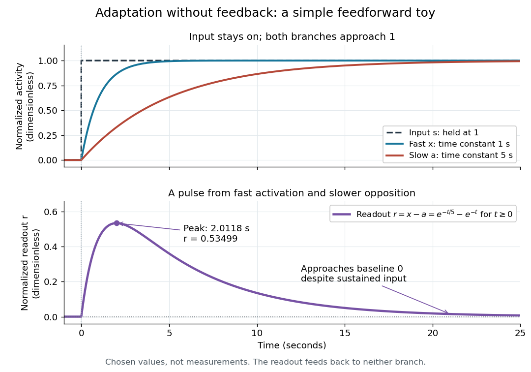
Find the pulse maximum by differentiating the exponential functions. With numerical time in seconds, the derivative isThe stationary condition is $e^{-4t/5}=1/5$, so the natural logarithm givesBefore this time the derivative is positive; afterwards it is negative. Together with $r(0)=0$ and ${\lim }_{t\to \infty }r(t)=0$, this proves that it is the unique pulse maximum. As another numerical check, at $t=10$ seconds $x\simeq 0.999955$, $a\simeq 0.864665$ and $r\simeq 0.135290$: the slow branch is still catching up.

The subtraction $r=x-a$ is a mathematical readout, not a claim that an actual chemical concentration equals this difference for arbitrary inputs. Nonnegativity was established only for the specified upward step; other input histories can give a negative signed readout. Complete signaling adaptation here also relies on equal eventual branch gains: changing the readout to $r=x-0.9a$ leaves $r_{\ast }=0.1$ for $s=1$. This toy illustrates cancellation and different time constants; it does not establish molecular implementation or robustness to arbitrary parameter changes. Ma and colleagues' 2009 study separately analyzed biochemical mathematical models with negative feedback and incoherent feedforward loops, identifying additional conditions for signaling adaptation in those models. ^[ref]

A historical connection to feedback control comes from Yi, Huang, Simon and Doyle's 2000 analysis of a bacterial chemotaxis model. They identified integral action in its regulation of receptor activity: accumulated deviations alter a slower adjustment, which in turn changes the measured activity. At a stationary state, an adjustment that integrates a nonzero error cannot remain constant, explaining how zero error can follow. Their conclusion depended on stated biochemical assumptions and stable behavior; it was not a claim that every biological cell uses that mechanism. A transient pulse alone, as the incoherent feedforward loop toy shows, cannot identify the underlying signaling feedback architecture. ^[ref]

Signaling feedback returns the effect of a downstream event to an earlier stage of signal transduction, closing a loop analogous to feedback control. Trace the causal arrows: if an earlier relay activates a later relay and the later relay changes the earlier relay's activity, the return path closes the loop. Negative feedback opposes the initiating change; positive feedback reinforces it. Signaling feedback is a possible property of signal transduction, not a requirement of every pathway.

For a schematic example, let relay $A$ activate relay $B$. If $B$ inhibits $A$, increased $A$ eventually produces an opposing influence: negative feedback. If $B$ activates $A$, increased $A$ produces a reinforcing influence: positive feedback. These signs describe effects on activity, rather than the direction in which molecules travel. A closed loop containing two inhibitions can have positive feedback, because inhibiting an inhibitor reinforces the original change. The sign belongs to the whole loop.

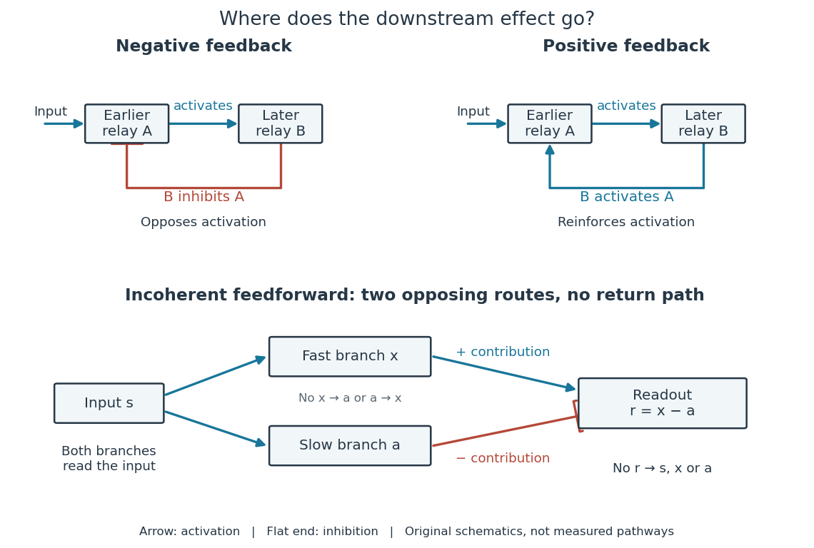
Negative feedback can restrain excessive activation and help preserve a usable range of responses. Positive feedback can support a decisive transition: Alberts and colleagues describe an enzyme whose product increases its own activity. Such reinforcement can contribute to switchlike behavior, but a positive feedback arrow alone does not prove bistability. A different structure, an incoherent feedforward loop, sends opposing influences forward from the same input; inhibition there is not a downstream return. ^{[ref] [ref]}

A worked mathematical model shows why negative feedback does not automatically produce complete signaling adaptation. Let $s$ be a fixed normalized input, $r$ a normalized response, $g\ge 0$ a dimensionless feedback gain, and $\tau >0$ a time constant. Suppose response removal contributes $-r$ and a return proportional to the response contributes $-gr$. The ordinary differential equation isSetting the derivative to zero gives the equilibrium point $r_{\ast }=s/(1+g)$. A displacement $\delta r=r-r_{\ast }$ obeys $\tau d(\delta r)/dt=-(1+g)\delta r$, so its decaying exponential function establishes asymptotic stability. For a unit input switched on at $t=0$, initial condition $r(0)=0$, $g=2$ and $\tau =1$ second,The negative feedback reduces the eventual response from $1$ to $1/3$, but this response rises monotonically and never returns to its zero baseline. Attenuation and complete signaling adaptation are different properties. This deliberately simple mathematical model specifies no molecular pathway; integral action provides a contrasting way to remove a lasting offset in a stable feedback control system. ^[ref]

An ideal voltage source $V_0$ and series resistor $R_1$ feed parallel branches $L$ and $R_2$. Thévenin's theorem gives $R_{\mathrm{th}}=R_1{R}_2/(R_1+R_2)$ and $V_{\mathrm{th}}=V_0{R}_2/(R_1+R_2)$. Starting with zero inductor current, $i_L=(V_0/R_1)(1-e^{-t/\tau })$ and $i_2=V_0{e}^{-t/\tau }/(R_1+R_2)$. Switch-on heat in $R_2$ is $L{V}_0^2/[2R_1(R_1+R_2)]$. Disconnecting the source leaves the stored magnetic energy $L{i}_L^2/2$ to dissipate through $R_2$, with time constant $L/R_2$.

A spark gap can rapidly discharge a charged capacitor through an inductor. After excitation, the stored energy runs down through Joule heating, radiation and other losses. A key held down can permit repeated discharges: each discharge starts a damped train of rapid oscillations. The spark repetition frequency, the electrical oscillation frequency within each train, and the rate of keyed symbols are different quantities. Repetition does not make each train a maintained sinusoid.

An original lumped model replaces the conducting spark gap and other losses by a constant total electrical resistance $R>0$ in an isolated series RLC circuit. For electric charge $q$ on the capacitor, the Kirchhoff cycle law givesFor $Q>1/2$, its characteristic roots are $-\alpha \pm \mathrm{i}{\omega }_d$, with ${\omega }_d=\sqrt{{\omega }_0^2-{\alpha }^2}$, proving the stated damped form. The electric current $\dot{q}$ has the same exponential decay scale. Its wave envelope falls by $\exp (-2\pi \alpha /{\omega }_d)$ per cycle; the energy envelope falls twice as fast in the exponent. A maintained sinusoid instead requires continuing input power balancing losses.

With $L=5\mathrm{mH}$, $C=2\mathrm{nF}$ and $R=100\Omega$, the model gives $f_0={\omega }_0/(2\pi )=50.329\mathrm{kHz}$, Q factor $Q=15.811$, amplitude time constant $1/\alpha =100\mu \mathrm{s}$, and damped frequency ${\omega }_d/(2\pi )=50.304\mathrm{kHz}$. These are chosen component values. A real spark gap switches nonlinearly, an antenna radiates, and coupling exchanges energy between circuits; one constant-$R$ free decay does not model the complete transmitter. Rapid damping also broadens the frequency spectrum, which helps explain why short trains make sharp receiver selection difficult.

A synaptic potential is a postsynaptic change in membrane potential caused by activity at a synapse. Unlike the regenerative action potential, a passive synaptic potential is graded: its size depends on input strength, the initial membrane potential and the receiving cell membrane's properties. Local voltage changes can decay before reaching the soma; their timing and overlap help determine whether an action potential follows. See Ion Channels and the Electrical Properties of Membranes.

Depolarization means that the interior becomes less negative relative to the exterior; hyperpolarization means that it becomes more negative. Excitation and inhibition instead describe whether an input promotes or opposes postsynaptic action potential generation. An inhibitory postsynaptic potential can be depolarizing, and shunting inhibition can occur with no voltage change at rest. The receptor, permeating ions, ionic gradients and reversal potential matter. See Purves and colleagues: excitation, inhibition and depolarizing inhibition.

A worked passive model treats the receiving membrane as one compartment with capacitance $C>0$, leak conductance $g_L>0$, and activated synaptic conductances $g_e,g_i\ge 0$:All electric currents are inward-positive. Each term $g(E-V)$ vanishes at its reversal potential $E$; $\mathrm{nS}\times \mathrm{mV}=\mathrm{pA}$. With constant parameters, the ordinary differential equation hasHere $G$ is total conductance, $1/G$ is effective electrical resistance, $V_{\infty }$ is the steady state and $\tau$ the time constant. Without imposed electric current, $V_{\infty }$ is a conductance-weighted average of the reversal potentials. This approximation omits spatial structure, changing ionic gradients and active voltage-gated ion channels; it calculates passive voltage responses, not actual action potential waveforms. See 3.1 Synapses for the mechanism behind the terms; the inward-positive convention here reverses that source's synaptic-current sign.

Take the same illustrative leak and capacitance as under shunting inhibition, start at $V(0)=-65\mathrm{mV}$ and set $I_{\mathrm{ext}}=0$. Opening $g_e=2\mathrm{nS}$ with $E_e=0\mathrm{mV}$ gives $V_{\infty }=-650/12\simeq -54.167\mathrm{mV}$ and $\tau \simeq 16.667\mathrm{ms}$. Its initial inward electric current is $2(0+65)=130\mathrm{pA}$. Adding $g_i=20\mathrm{nS}$ with $E_i=-65\mathrm{mV}$ changes $V_{\infty }$ to $(-650-1300)/32=-60.9375\mathrm{mV}$ and $\tau =6.25\mathrm{ms}$. This is shunting inhibition of the same excitatory drive.

For comparison, $g_i=20\mathrm{nS}$ with $E_i=-75\mathrm{mV}$ alone gives $V_{\infty }\simeq -71.667\mathrm{mV}$: hyperpolarization. With $E_i=-60\mathrm{mV}$ instead, it alone gives $V_{\infty }\simeq -61.667\mathrm{mV}$: depolarization. Yet adding this depolarizing conductance to the $g_e=2\mathrm{nS}$ excitatory drive lowers that drive's $V_{\infty }$ from $-54.167$ to $(-650-1200)/32=-57.8125\mathrm{mV}$. At an illustrative firing threshold $V=-50\mathrm{mV}$, its electric current is $20(-60+50)=-200\mathrm{pA}$, opposing threshold approach. The combined trace initially rises faster than the excitatory drive alone, before settling below it. Thus the sign of a voltage change at rest alone does not determine excitation or inhibition; a claim about firing must specify input strength, timing and the neuron's state.

This deliberately synthetic differential equation model illustrates response direction and lag. Every plotted number is chosen for teaching; none is a biological measurement or a fitted human parameter. Let externally prescribed, dimensionless $g>0$ represent a glucose stimulus relative to a reference. Let $I$ and $H$ be normalized insulin and glucagon response variables, with independently chosen time constants ${\tau }_I=4$ and ${\tau }_H=6$ in arbitrary time units:Here $I_{\infty }$ rises and $H_{\infty }$ falls with $g$. Their targets add to one by construction; the evolving $I+H$ need not equal one because their time constants differ. Start with $g=1$ and $I=H=1/2$. Set $g=1.6$ from $t=10$ to $40$, $g=0.65$ from $t=40$ to $70$, and $g=1$ otherwise. Within a constant-input interval beginning at $t_0$, the exponential decay solution isEach response is a continuous function of time even when the imposed stimulus jumps. The chosen starting values stay between zero and one, since each solution is a weighted arithmetic mean of its interval's starting value and target.

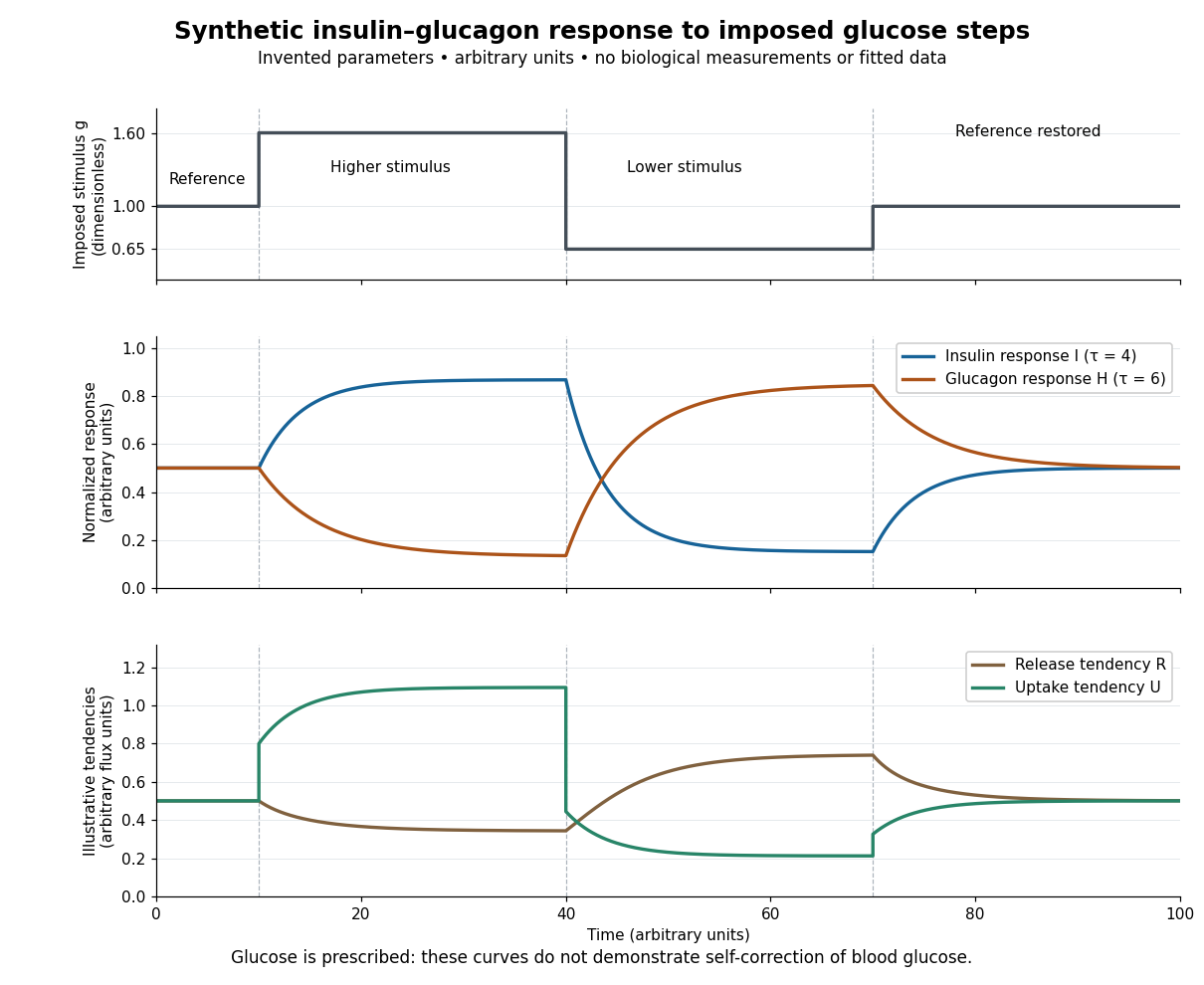
For an illustrative downstream comparison, define release tendency $R=0.3+0.6H/(1+I)$ and uptake tendency $U=(0.25+0.5I)g$, in the same arbitrary flux units. At the reference target, $R=U=0.5$. At the high-stimulus targets, $R\approx 0.343$ and $U\approx 1.094$; at the low-stimulus targets, $R\approx 0.742$ and $U\approx 0.212$. These chosen functions encode greater uptake with insulin and greater release with glucagon, moderated by insulin; they are not established enzyme kinetics. The $g$ trace is imposed externally, so the figure does not demonstrate self-correction of blood glucose. A closed model would also need a conservation of mass equation, nutrient input, finite glycogen stores, and additional tissue interactions. The qualitative restoring loops are shown separately in the insulin circuit.