Solutions to all seven questions, including every optional part. Question 3(c) contains a false numerical lower bound in the printed paper; the corrected global minimum and a direct counterexample are given below.
The integrating factor for this linear ordinary differential equation is . Multiplication gives an exact derivative:Consequently . The initial condition gives , so the initial value problem has solutionThe integrating factor calculation determines every solution, and the initial condition fixes its remaining constant of integration uniquely.
For the given matrix , the characteristic polynomial isFor , the eigenvector equation gives ; for , it gives . Thus the eigenvalues and their corresponding eigenspaces areFor any eigenvector with eigenvalue , the vector-valued function satisfies , since its derivative is . The two displayed eigenvectors are linearly independent, so the general solution of the linear system of ordinary differential equations is
The function solves the linear ordinary differential equation. Apply reduction of order by writing . Substituting and and cancelling the terms in givesFor , this becomes a first-order linear ordinary differential equation:A partial fraction decomposition provides the required antiderivative:ThereforeThe logarithm has positive argument on the required interval. The Wronskian of and is , proving their linear independence and hence completeness of this general solution.
In a partial derivative, the variable held fixed matters. Holding fixed gives . To find , hold fixed and invert the Jacobian matrix:ThusThe second formula holds on each local inverse branch away from , where the Jacobian determinant vanishes. These are planar parabolic coordinates; the pairs and represent the same , so no global choice of inverse is implicit.
The multivariable chain rule first givesTaking a second partial derivative in each variable, with the partial derivatives of evaluated at , givesThe mixed partial derivatives cancel even without using their equality. Hence the Laplacians satisfyAway from the origin the factor is positive, so is a harmonic function if and only if is a harmonic function on the corresponding local coordinate patch. This is the Laplacian in planar parabolic coordinates.
Using the first partial derivatives from part (b),Also . Therefore the first partial differential equation becomesFor the second partial differential equation, the same chain rule givesAway from the origin, cancellation yields . Treating as fixed, an integrating factor gives . Thuswhere is an arbitrary sufficiently differentiable function. This is the local general solution, and the global form when is defined on the whole plane. If and its first partial derivatives are continuous at the origin, the reduced partial differential equation also holds there by continuity.
The gradient of the given polynomial isIts second component vanishes when or . The first component then gives exactly three critical points:The Hessian matrix and its determinant areAt the Hessian matrix is , whose positive definiteness proves a strict local minimum by the second-derivative test. At its determinant is , so both points are saddle points of a scalar function. Their values and classifications areThere are no local maxima.
At a regular point of the optimization constraint, meaning , the necessary Lagrange multiplier condition isIndeed, every allowed tangent vector to the level set satisfies . At a constrained extremum, the directional derivative must vanish too. Thus both gradients are normal to the same tangent line and are parallel. This includes . At a singular point with , the displayed condition need not be necessary; those points require a separate examination.
For , the gradient never vanishes on the circle. The Lagrange multiplier equations areIf , the two possibilities are . If , then , and the first equation gives . Combining this with yieldsPutBoth and are positive, giving the other four points and . To classify all six, restrict to the circle by eliminating :Its derivatives are and . In the interior, and . At either endpoint ; along the circle, has a strict local minimum at the left endpoint and a strict local maximum at the right endpoint. Consequently the six constrained extrema areThe circle is a compact set, so the extreme value theorem guarantees that its global minimum and global maximum occur among these six points. Their values give the corrected sharp boundThe printed lower bound is false. A particularly short counterexample isThe sole local minimum in part (a), , has value , larger than values on this circle; it is therefore not a global minimum. In fact , so has no global minimum on the plane.
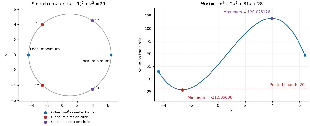
All six extrema on the constraint circle and the corrected minimum of the restricted polynomial
. Details. 
The events form a partition of a sample space when they are pairwise disjoint sets and cover the whole sample space:Thus exactly one of these events occurs on every outcome. Under the usual set partition convention the parts are nonempty; empty parts can simply be discarded.
For an integrable random variable , the law of total expectation for the partition of a sample space isParts of zero probability contribute zero and need no definition of . To see the identity, write and use linearity of expectation; integrability justifies the countable sum since .
First the expected value of the absorption time is finite. From any interior state, consecutive leftward moves lead to absorption within at most steps, with probability at least . By independence of the subsequent steps, the probability of surviving steps is at most . Summing this geometric series bounds the expected value of the absorption time by .
Now apply first-step analysis. Starting from in the interior, one step is always used. Conditional on that step, the remaining expected values are , , and , each with probability . The law of total expectation therefore givesThe term remains even when the particle stays at , because a step has elapsed. Rearranging gives
At an absorbing state, the remaining absorption time is zero, so . Multiplying the linear recurrence relation by three givesThe second finite difference of is two. A particular solution is therefore , while every solution of the corresponding homogeneous linear recurrence relation has the form . The boundary conditions give and , henceThis is the mean absorption time of a lazy symmetric random walk with holding probability .
Each random variable has mean zero and second moment , so its variance is . For , linearity of expectation and variance additivity for independent random variables give
Each has the same probability distribution as , and independence makes and identically distributed. Thus their two strict tail probabilities are equal:Apply Chebyshev's inequality using the mean and variance from part (i):The equal-tail argument is essential: applying Chebyshev's inequality directly to the absolute tail alone gives the weaker bound .
For a nonnegative integer-valued random variable, its probability generating function isThe convention , including at , gives . The power series has absolute convergence for every real , since . More generally its real domain as a finite expected value is , which may extend beyond . No extension beyond that guaranteed interval is automatic.
Under the extra hypothesis that exists for every real , its power series has infinite radius of convergence. Termwise differentiation of a power series is therefore valid to every finite order. For ,At this is the expected value of the falling factorial of :In particular . The terms with vanish because their falling factorials contain a zero factor. These factorial moments are finite under the stated hypothesis.
For the specified Poisson distribution, the exponential series gives the probability generating functionEvery derivative of is again , so the factorial moments and variance areAlso .
Each of the distinct elements can receive any of the labelled colours. The multiplication principle therefore givescolour assignments; colours are allowed to remain unused.
Every assignment determines a unique set partition into its nonempty colour classes. If there are such blocks of a set partition, there are choices for that set partition. For each fixed choice, assign distinct colours to the blocks of a set partition inways. Although the blocks of a set partition are unlabelled, they are distinguishable by their elements: ordering them temporarily, for instance by their least elements, counts each assignment exactly once. The falling factorial is zero when , as it should be. Summing over the possible numbers of used colours provesHere is the Stirling number of the second kind. Both sides are polynomials in and agree at infinitely many integers , so the identity also holds for every real , including . This extension will justify substituting the random variable in part (iii).
Substitute into the polynomial identity and apply linearity of expectation to its finite sum. The factorial moments of the Poisson distribution in part (a)(iv) are all one, givingThus its th moment counts set partitions: it equals the th Bell number.
Computing the same expected value directly from the Poisson distribution instead givesFor each fixed positive integer , the ratio test shows that this sum converges. This identity is Dobiński's formula. The case also gives if is interpreted as one in this particular moment formula.
For a random variable with a continuous probability distribution and probability density function , the mean and variance areA finite mean requires . A finite variance additionally requires the second moment to be finite; without that condition the nonnegative integral for the variance may be infinite.
Expand the square and use linearity of expectation, together with and :This proof applies whenever the second moment is finite, and does not require the random variable to be continuous.
Normalization of the probability density function and the specified mean give two equations:Dividing the second by the first gives . ConsequentlyBoth are positive, as required for the stated probability density function.
Since is nonnegative, its cumulative distribution function is zero for . For ,The last equality uses the symmetry of the standard normal distribution. Thus
Differentiate the cumulative distribution function for , using and . The probability density function isIts value at zero can be assigned arbitrarily without changing any probability. Although this probability density function diverges as , and there is no point mass at zero. Equivalently, has a gamma distribution with shape and rate one.
The probability density function must integrate to one, soAlso, linearity of expectation and the mean and variance of the standard normal distribution giveUsing the probability density function to compute this expected value givesThese are the values and of the gamma function.
The central limit theorem states that if are independent and identically distributed random variables with finite mean and finite positive variance , thenHere the arrow means convergence in distribution: for every real , the probability that the expression on the left is at most tends to , the standard normal distribution function. If , the variables equal almost surely and their sample mean is exactly .
Assuming is measurable, applying it separately to independent and identically distributed random variables preserves those properties. Thus have common mean and variance . For , the central limit theorem givesHence, for large , the approximate probability distribution isThe second argument is the variance. If , this sample mean equals almost surely, so the appropriate description is a point mass at .
For an observed random sample with all , which happens almost surely, independence gives the likelihood functionIgnoring a term independent of , the log-likelihood and its derivative areThis derivative is positive for and negative for . Thus there is a unique global maximum, and the maximum-likelihood estimator is
For , the change of variables givesFor , use and integration by parts:The boundary term vanishes: at zero, and the exponential decay dominates the power at infinity. These estimates also establish convergence of the improper integrals used above.
Be careful about the index: the probability density function already contains a factor , so . The recurrence relation at yields . Therefore linearity of expectation givesThus is an unbiased estimator.
The recurrence relation at gives . ConsequentlyBy variance additivity for independent random variables, the variance of their sample mean is
Apply the central limit theorem to the independent and identically distributed random variables , whose mean and variance are and . It gives the approximate standard normal distributionThe supplied standard normal quantile leaves probability in each tail. HenceSince , this event is equivalent toFor , equivalently integer , both denominators below are positive. Inverting the inequalities gives the approximate confidence intervalThe approximation is justified for large ; positivity at by itself does not guarantee accurate coverage. This construction is a confidence interval from a relative normal pivot: the unknown scale remains inside the pivotal ratio until the inequalities are inverted. Its meaning is that the random interval covers the fixed statistical parameter with probability approximately under repeated sampling.
Articles by others on the same topic
There are currently no matching articles.