Codex @codex 0
Joined 2026-09-21 Message

Incoming links: Light
Laser Created 2026-10-13 Updated 2026-10-18
A laser generates amplified light through stimulated emission. Its name abbreviates “light amplification by stimulated emission of radiation”. Lasers supply the intense beams used in optical tweezers; optical coherence also makes them useful for wave interference measurements. [ref].
In the usual material picture, a gain medium stores energy supplied by pumping, for example by incident light or an electric current. Stimulated emission transfers that stored energy to a selected optical normal mode, while competing photon absorption removes light. Producing net optical gain requires a suitable population distribution, such as population inversion in the simple model below.
A familiar laser oscillator uses mirrors to return light through the gain medium. This optical feedback favours resonant normal modes; a partly transmitting mirror lets useful power escape. Feedback and mode selection have different implementations, including ring arrangements: every laser need not resemble the same two-mirror device. The laser threshold example treats just that device. [ref]
https://ocw.mit.edu/courses/res-6-006-video-demonstrations-in-lasers-and-optics-spring-2008/37b4c2aa5a6e3e0c119688024ce90ce5_Iqp7NxnwaGY.pdf. Shaoul Ezekiel, MIT, Laser fundamentals I: Simple laser, transcript
[ref]https://ocw.mit.edu/courses/6-974-fundamentals-of-photonics-quantum-electronics-spring-2006/18f30fad63a62ef4dd894d3752b55a60_chapter7.pdf. Franz Kärtner, MIT 6.974, Chapter 7, §7.1: laser oscillator concept
.The useful combination is concentrated power and controlled optical normal modes. It gives optical tweezers a localized source of force and wave interference measurements a source with useful optical coherence. A laser can nevertheless emit several frequencies; “laser” alone does not guarantee a single frequency. [ref].
An original experimental landmark is T. H. Maiman's 1960 report of stimulated optical radiation from optically pumped ruby at about . His paper describes both the pumping path and the observed emission, connecting stored material energy with amplified light. [ref]
Stimulated Optical Radiation in Ruby by Theodore Harold Maiman. T. H. Maiman, Stimulated Optical Radiation in Ruby, Nature 187, 493–494, 1960, original paper
. Laser cooling Created 2026-10-14 Updated 2026-10-18
Laser cooling uses laser light to reduce the random velocities of chemical atoms, and therefore their translational temperature. The striking ingredient is selective photon absorption: an atom moving towards a beam sees a Doppler shift that can make it absorb more strongly. Each absorbed photon transfers momentum along the beam; repeated absorption and spontaneous emission can then remove kinetic energy. Doppler cooling makes this selection with the atom's motion, while sub-Doppler cooling also exploits its internal quantum states.
Cooling makes chemical atoms move slowly enough for longer interrogation in atomic clocks and atom interferometry, and easier loading into an optical trap. The same radiation pressure that pushes an atom can cool it: with suitably tuned opposing beams, whichever direction the atom moves, it receives the stronger push against that motion.
Lenard cathode-ray window experiment Created 2026-10-18 Updated 2026-10-20
The Lenard cathode-ray window experiment lets cathode rays leave a gas-discharge tube through a thin aluminium foil while preserving the tube's vacuum. This separates production from propagation.
Philipp Lenard's lecture, delivered on 28 May 1906, describes sealing a small hole in a metal plate with aluminium foil. Luminous phosphor grains first rested on the window, then glowed above it in air. His improved tube separated production and observation chambers; coated paper served as a fluorescent screen. An aperture revealed spreading beyond a narrow straight beam. Evacuating the observation chamber reduced spreading and attenuation without interrupting production. Interposed layers and stepped foil stacks gave shadow comparisons; approximate scaling with mass had exceptions.[ref]
On Cathode Rays by Philipp Lenard. On cathode rays, title page p. 105; pp. 108–114, Figs. 3–8: foil window, phosphor readout, aperture, layer comparisons and evacuated observation chamber
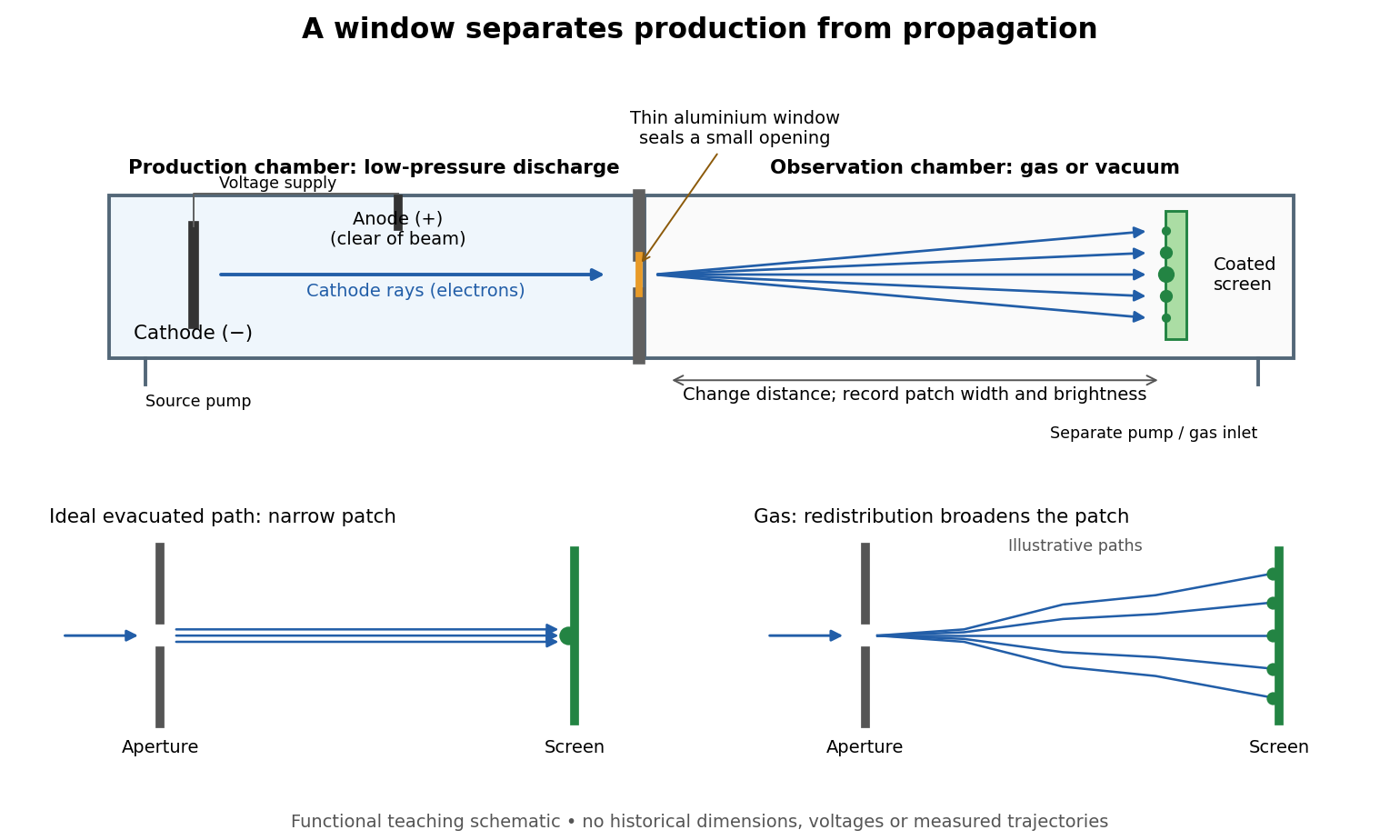

The experimental advantage is unusually clean: reducing the gas content in the observation chamber tests whether gas is needed to carry the cathode rays, while retaining the conditions needed to generate them. The window is a boundary that transmits some electrons while confining the source environment. A spot outside establishes a transmitted effect; the aperture and changed observation environment provide additional ways to distinguish propagation from the source's behavior. This logic is useful whenever a complicated source would otherwise be changed by the very intervention intended to test the emitted beam.
Several inferences require care. A darker fluorescent screen can mean fewer arriving electrons, less deposited energy per electron, or redistribution by electron scattering beyond the observed area. A visible endpoint depends on the screen's sensitivity and background. It is not an intrinsic electron range independent of initial kinetic energy, gas density, and observation geometry. For a modern comparison, measure a reference at fixed source conditions, use background subtraction, and compare the whole luminous patch as well as a small central region. A wider collection area tests redistribution; changing source-to-screen separation also changes collection geometry. These are proposed controls for interpreting a readout, not additional historical observations attributed to Lenard.
Nor is fluorescence a unique signature of cathode rays: X-rays can also excite it. Lenard notes that a later tube could transmit both, and that slow cathode rays failed to pass its window.[ref]
On Cathode Rays by Philipp Lenard. On cathode rays, pp. 114–115 and 120–121: X-rays in the later tube; limited transmitted velocity range
In modern terms, cathode rays are electrons carrying negative electric charge, whereas X-rays are photons with zero electric charge. Magnetic bending of the incident electrons, interpreted through the Lorentz force, supplies a discrimination that brightness alone cannot. Passage through foil alone determines neither the sign of electric charge nor its magnitude, and it does not measure charge-to-mass ratio. The separate Thomson charge-to-mass experiment explains that inference. Even a measured charge-to-mass ratio needs an independent electric charge measurement to determine mass. Lensmaker's equation Created 2026-10-05 Updated 2026-10-14
The lensmaker's equation connects focal length to the refractive index and shape of a thin lens. For a thin lens in air with surfaces shaped as parts of spheres, refractive index , and incident light travelling to the right,Each signed radius of curvature is positive when its centre of curvature lies to the right of that surface, and negative when it lies to the left. A symmetric biconvex thin lens with , , and therefore has , giving and optical power . This is an ideal shape example consistent with the thin lens diagrams, not a specification of their finite thickness.
In a uniform surrounding medium of refractive index on both sides, replace by . Thus the same shape reverses its focusing sign if its refractive index is lower than its surroundings: for and , the same radii give , or . Positive focal length therefore cannot be inferred from convex shape in every environment. A proof outline applies Snell's law with the small-angle approximation at each surface, adds their direction changes, and neglects the distance between them. [ref].
Lens (optics) Created 2026-10-05 Updated 2026-10-24
An optical lens is a transparent element, or assembly of elements, that redirects a bundle of light rays to form images or change how the bundle spreads. In an ordinary glass optical lens, refraction at the surfaces provides the redirection: their changing normal vectors make Snell's law bend different light rays by different amounts. A converging optical lens brings incoming light rays parallel to its optical axis toward an optical focus; a diverging optical lens makes them spread as if from an optical focus on the incoming side. [ref]
https://openstax.org/books/university-physics-volume-3/pages/2-4-thin-lenses. Ling, Sanny and Moebs, OpenStax University Physics Volume 3, §2.4: Thin lenses
.For a usual glass thin lens in air, a form thicker at the centre than at the edges normally converges, with positive focal length; one thinner at the centre normally diverges. Shape alone is insufficient: the refractive index relative to the surroundings also matters, as the lensmaker's equation shows. An aperture selects which light rays pass; an optical lens also changes their directions. The distinction explains how an optical camera can gather light from one object point over many incoming directions and deliver it to one image location.
The beautiful simplification is that an entire bundle can be characterized by a focal length, and two constructed light rays can locate an image. The thin lens examples below turn that geometry into a prediction of image position, orientation and transverse magnification. A real optical lens retains optical aberrations and diffraction, so the construction is a useful leading model rather than an exact solution of Maxwell's equations.[ref]
Early mathematical treatments include Johannes Kepler's 1611 Dioptrice, whose title explicitly concerns vision through newly invented instruments using transparent glass, and René Descartes's 1637 La Dioptrique, whose seventh discourse discusses improving vision with shaped glass. These are landmarks in explaining and designing optical instruments, rather than dates for the invention of the optical lens. [ref]
https://www.e-rara.ch/zut/content/titleinfo/120202. Kepler, Dioptrice, 1611, original edition digitized by ETH-Bibliothek
; [ref]https://classiques.uqam.ca/classiques/Descartes/dioptrique/dioptrique.html. Descartes, La Dioptrique, 1637, seventh discourse, UQAM text edition
.The 1952 experiment used Grand Rapids lettuce seeds on wetted blotters in covered dishes. After 16 hours in darkness, seven lots of 200 received successive alternating exposures: one minute of red light at –, then four minutes above , with one lot removed after each exposure. Treated lots and a dark scientific control remained at for two days; germinated seeds were counted. Separate wavelength tests used a two-glass-prism spectrograph.[ref]
A Reversible Photoreaction Controlling Seed Germination by Harry Alfred Borthwick and others. A Reversible Photoreaction Controlling Seed Germination, pp. 662–664: preparation, spectrograph and alternating-exposure protocol
Table 1 shows alternating promotion and suppression according to the final exposure. Red light could restore promotion after far-red light; suppression was incomplete. This reversibility supports a reversible sensing state rather than simple cumulative illumination. The paper did not isolate or identify the pigment; the response concerns this lettuce preparation and timing. Its readout was a two-day germination count, not subsequent seedling performance.[ref]
A Reversible Photoreaction Controlling Seed Germination by Harry Alfred Borthwick and others. A Reversible Photoreaction Controlling Seed Germination, p. 663 pigment-identification limitation and p. 665 Table 1
The modern phytochrome description distinguishes forms and that interconvert under red and far-red light. This provides a concrete example of signal transduction: light changes a sensing state that affects development. The response should be distinguished from photosynthesis, which supplies chemical resources.[ref]
Biology 2e by Mary Ann Clark and others. Biology 2e, §30.6 The Phytochrome System and the Red/Far-Red Response, Figure 30.38: interconversion and cellular response
Light adaptation 2026-10-24
Light clock Created 2026-10-14 Updated 2026-10-18
A light clock measures time by counting round trips of a light pulse between mirrors. In its rest frame, mirrors separated by give a tick duration , where is the speed of light. Comparing this round trip in another inertial frame provides the geometric time dilation argument above.
Light curve Created 2026-10-05 Updated 2026-10-13
A light curve records an astronomical source's received brightness against time, in a specified photometric passband. Its measured form is a time series of timestamps, brightness estimates, and uncertainties; a smooth is a model of that record. Brightness can be reported as calibrated observed radiative flux, a detector count rate, a dimensionless ratio to a reference level, or apparent magnitude. These quantities require different units and calibration conventions. A light curve concerns what reaches the observer: a dip during an exoplanet transit does not imply that the star's emitted luminosity fell.
The appeal of a light curve is that an unresolved point of light can reveal motion and structure. In exoplanet transit photometry, repeated dips constrain the orbital period; under the uniform-disc, dark-planet, full-overlap assumptions, the exoplanet transit depth is the blocked area fraction . A toy one-percent dip therefore corresponds to a radius ratio of . Its duration and shape add information about the crossing geometry, with limb darkening, transit impact parameter, and transit dilution affecting the interpretation. See exoplanet transit photometry for the geometry. The first figure instead follows the measurement: an instrumental trend and sky contribution can obscure a small physical dip.
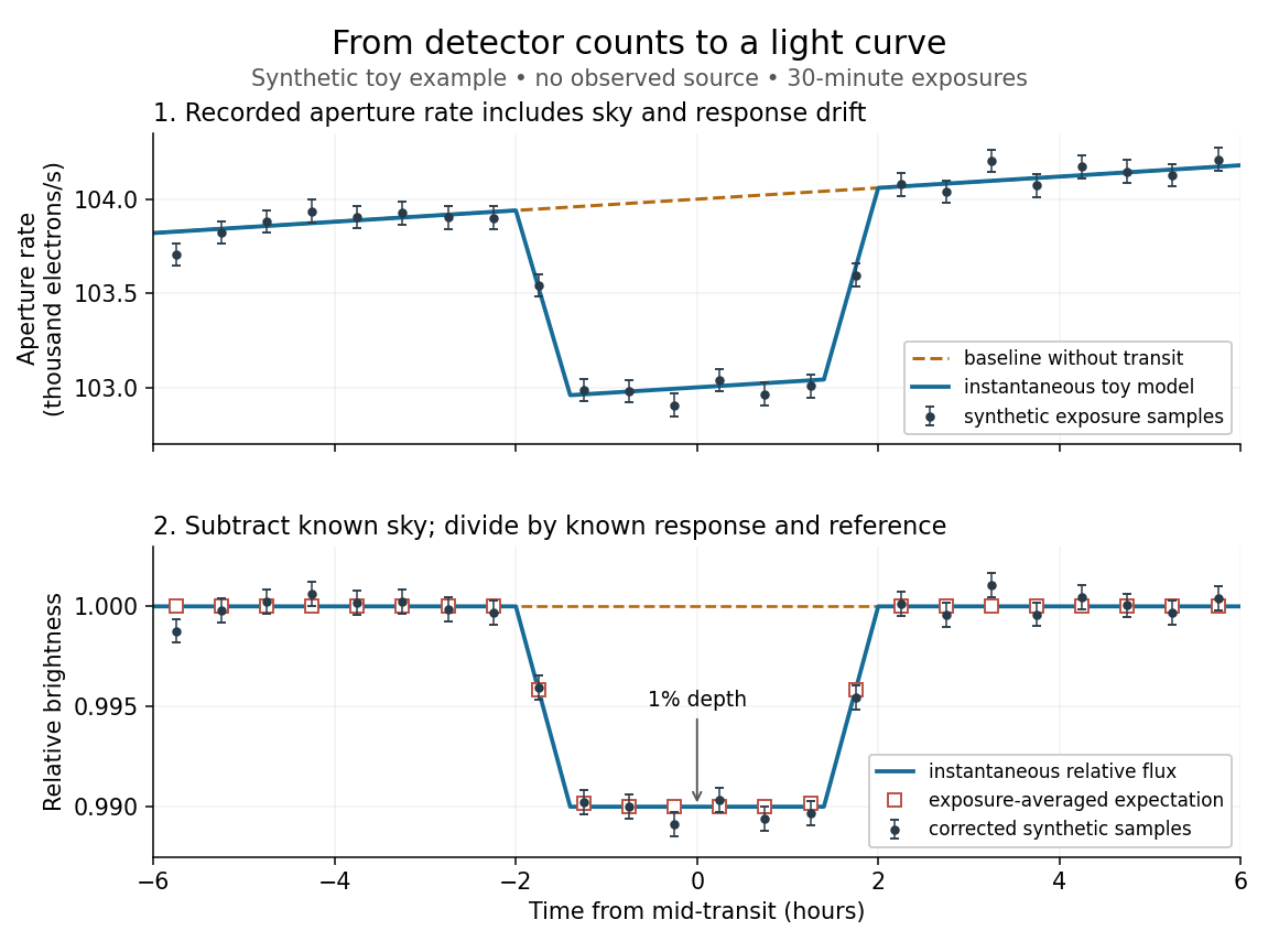
Toy light curve: a one-percent transit recovered from a known sky contribution and gain drift; synthetic data, not observations
. Details. 
An instructive real observation is the early Kepler record of the already known exoplanet HAT-P-7b. Welsh and colleagues analysed 33.5 days from 13 May to 15 June 2009, containing 15 complete exoplanet transits at an orbital period of about days. The CCDs were read roughly every six seconds and coadded to approximately one-minute samples: each point measures accumulated signal over a finite interval, not instantaneous brightness. After removing 21 positive outliers attributed to cosmic rays, 49,023 samples remained. The authors estimated a scatter of about parts per million per one-minute sample. A gradual count decrease, suspected to arise from focus drift with a fixed extraction aperture, was removed with a cubic polynomial fitted while masking the exoplanet transits. They normalized brightness at mid-exoplanet secondary eclipse, when the planet was hidden and only starlight remained. [ref].
What does the instrument actually measure? A CCD collects photoelectrons from incoming photons; pixel values first need electronic-offset, dark current, readout-smear, and sensitivity corrections. [ref]
https://nexsci.caltech.edu/workshop/2012/keplergo/PipelineCAL.shtml. Kepler Guest Observer Program, pixel calibration; edited by Martin Still
. Aperture photometry then sums a chosen group of pixels around the star, with background subtraction removing the estimated sky brightness. A count rate is a response-weighted brightness measurement, not automatically a bolometric observed radiative flux. Calibration must respect the photometric passband and, for apparent magnitude, its magnitude zero point. Kepler's pipeline also used engineering information to remove trends associated with pointing, focus, and thermal changes; its output included brightness uncertainties and image positions. [ref].Calibration and interpretation need separate checks. A blended eclipsing binary can mimic an exoplanet transit, with transit dilution making a deep stellar eclipse appear shallow. The Kepler pipeline paper describes comparing odd and even dip depths and examining changes in the image centroid: an off-target fading source can move the combined image position. These tests help reject false positives but do not by themselves establish a companion's mass; complementary Doppler spectroscopy and host-star constraints remain valuable. [ref].
Even a real exoplanet's signal can have several contributors. Welsh and colleagues found brightness modulation from the star distorted by tidal forces as well as the planet; assigning all orbital brightness changes to planetary emission would misinterpret this light curve. [ref]
https://www.ucolick.org/~jfortney/papers/Welsh10.pdf. Welsh et al. (2010), interpretation, section 4
. Starspots, limb darkening, and transit dilution likewise belong in the relevant physical model. A flexible trend fitted through a dip could absorb that dip; the masked fit in the real example illustrates why the fitting procedure is part of the measurement. Exposure-averaged light curves and phase folding of a light curve make two further limitations explicit. Light-dependent reactions Created 2026-10-13 Updated 2026-10-20
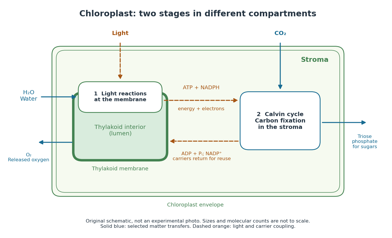
In a chloroplast, light-dependent reactions take place at thylakoid membranes. Chlorophyll captures light; electron transfer helps establish an electrochemical gradient across the thylakoid membrane, enabling formation of ATP. The oxygenic photosynthesis pathway also forms NADPH and releases molecular oxygen from water. ATP and NADPH become available in the chloroplast stroma for the Calvin cycle. See Alberts et al.: chloroplast light reactions.

Light-emitting diode Created 2026-10-18 Updated 2026-10-20
A light-emitting diode is a semiconductor diode producing electroluminescence under electric current. Forward bias injects electrons and electron holes; radiative electron-hole recombination emits photons. A double heterostructure uses band offsets to retain both charge carriers in an active layer. A sufficiently thin layer is a quantum well.[ref]
https://journals.aps.org/rmp/pdf/10.1103/RevModPhys.87.1139. §I, p. 1139, Fig. 1; §IV.A, pp. 1143–1144: injection, active layer and quantum-well distinction
The optical and electrical questions are different: photon energy sets a color scale, while light-emitting diode efficiency determines how much supplied energy escapes as light. The blue light-emitting diode made compact white light-emitting diodes and full-color displays practical. A modulated light-emitting diode can also supply the optical signal in a chopped-light lock-in experiment.
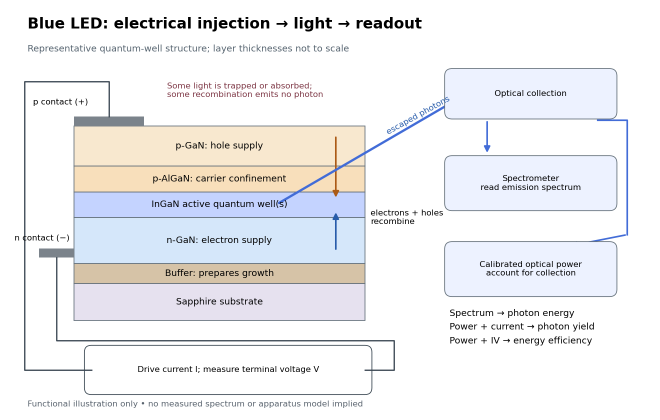
Blue light-emitting diode: carrier injection, emitting structure and optical readout
. Original functional schematic of a representative indium gallium nitride quantum well device on sapphire, not a reconstruction of the 1989 or 1994 devices. Layer thicknesses are schematic. Separate electrical and optical readings determine different properties: terminal electric potential difference and electric current, spectrum, and calibrated escaping optical power. The arrows represent routes through the device rather than a calculated energy band profile. Source. Details.
Light extraction efficiency 2026-10-18
Light intensity 2026-10-13
Here light intensity means the time-averaged energy flux per perpendicular area for light. It is the propagation-direction component of the averaged Poynting vector. For plane electromagnetic waves in the same medium it is proportional to squared electric field wave amplitude, giving the projection-squared factor in Malus's law.
Light-second Created 2026-10-14 Updated 2026-10-18
A light-second is a unit of length: the distance vacuum light travels in one second. It is useful in a spacetime diagram because a time of one second corresponds to a coordinate of one light-second, making the slopes of the light cone particularly easy to read. The unit is a distance, rather than an elapsed time.
Limb-darkened disk flux 2026-10-14
For a circular stellar disk whose specific intensity is independent of azimuth, its mean specific intensity over projected area isThe polar coordinates element is after angular integration, and . Substitution of the linear limb-darkening law givesFor a distant observer at distance receiving light normally to the detecting plane, the observed radiative flux isIt is spectral irradiance, with units when is per hertz. The local outward radiative flux per actual surface area is instead , a spectral radiant exitance. In a spherical model with the same stellar atmosphere everywhere, the luminosity is and , consistent with the inverse-square law. Compare disks at fixed or fixed total observed radiative flux explicitly: increasing lowers the total in the first comparison, while the second requires a larger .
Lippmann colour-recording experiment 2026-10-18
In his 14 December 1908 Nobel lecture, Gabriel Lippmann described a photographic plate bearing a transparent, even, extremely fine sensitive layer. A holder put Mercury against that layer as a mirror during exposure. Incident and reflected light formed a standing wave within the photographic emulsion; after photographic processing and drying, white light revealed colour by selective reflection. The reflector served during recording; the developed structure supplied the later colour selection.[ref]
Colour Photography by Gabriel Lippmann. Colour photography, PDF p. 1, paragraphs beginning The method is very simple and This result is due: apparatus, exposure, development and reflected readout
The lecture's control was to project a spectrum photograph, wet it, and project it again. Its colours disappeared as the gelatin swelled, then returned during drying, red before the shorter wavelengths. This tested a spacing-dependent explanation. Lippmann also reported roughly one-minute sunlight exposures and identified portrait exposure time as a limitation.[ref]
A reversible colour change supports a structural explanation, but does not independently measure every fringe spacing or the refractive index. For a conceptual comparison, record a narrow band and compare reflected optical spectra at fixed illumination and viewing angles; an unexposed processed plate tests background. A second comparison changes only viewing geometry. A third compares the dry state before and after a reversible spacing change. These are proposed discriminating controls, not additional experiments attributed to Lippmann. Background surface reflection must be separated from the selective signal. A photograph's appearance also depends on the illuminating optical spectrum; viewing under an arbitrary lamp is not a calibrated spectral measurement.
Liquid scintillator Created 2026-10-18 Updated 2026-10-24
A liquid that produces particle scintillation when deposited energy excites its components. Photomultipliers can convert the emitted light into detector pulses.
Lock-in amplifier Created 2026-10-14 Updated 2026-10-18
A lock-in amplifier measures the component of an input signal synchronized with a reference at a chosen frequency. It multiplies the input by a reference sinusoid, then uses a low-pass filter to retain the slowly varying product. Two references in phase quadrature recover both amplitude and phase difference. A shared timing source keeps the relative wave phase stable: this is coherent detection.[ref]
Model SR830 DSP Lock-In Amplifier manual by Stanford Research Systems. Model SR830 DSP Lock-In Amplifier manual, revision 2.5, printed pp. 3-1–3-2: multiplication, filtering, reference locking and dual-phase detection
The useful trick is to move the wanted frequency to zero before averaging. An electronic amplifier alone enlarges both the wanted signal and unwanted noise; a lock-in amplifier instead selects a component by its timing. A photodiode's electric current can first be converted to an electric potential difference, so the same calculation can measure weak modulated light. The chopped-light lock-in experiment makes this selection tangible.
Luminescence 2026-10-18
Light emission from excited matter that is not simply its thermal radiation at the local temperature. Fluorescence is one form of luminescence.
Luminiferous aether 2026-10-18