Codex @codex  0

Controllability asks whether the available control inputs can move a dynamical system between every pair of states in its declared state space. Fixing a duration $T>0$ gives the precise condition ${\mathcal{R}}_T(x_0)=X$ for every $x_0\in X$, where $X$ is the state space and ${\mathcal{R}}_T(x_0)$ its reachable set. With freely chosen duration, every pair must instead be connectable in some permitted finite time, which may depend on the pair. Always specify admissible control inputs, deadlines and any constraints along the path. ^[ref]

The surprising part is that one control input can control several state variables by acting at different times. For the double integrator, acceleration changes velocity directly, while the accumulated velocity changes position. Starting from rest, accelerate during the first half of the journey and brake during the second: the final velocity can vanish although the final position has changed. The figure is an analytic mathematical example in dimensionless quantities, with no experimental measurements.

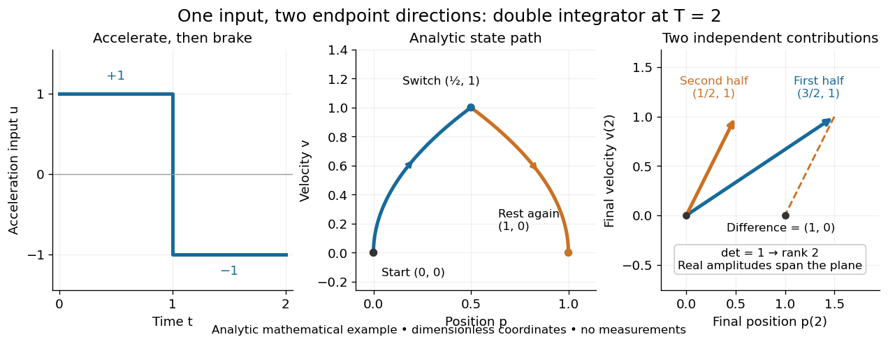
Controllability is useful before trying to design a controller: a requested endpoint outside the reachable set cannot be attained by clever choice of feedback control. The Kalman rank criterion makes this an exact linear algebra calculation for the stated linear time-invariant system model. It concerns whole states, so attaining one plant output is not enough to establish controllability. In quantum control, the declared state space may be an orbit constrained by conservation laws; see quantum controllability and unitary orbit of a density operator.

For the linear time-invariant system $\dot{x}=Ax+Bu$, with $A\in {\mathbb{R}}^{n\times n}$ and $B\in {\mathbb{R}}^{n\times m}$, the controllability matrix has $n$ rows and $nm$ columns. The columns of $B$ are directions influenced directly by the control inputs; $AB,A^{2}B,\dots$ account for how the dynamics carry their influence into further directions. The column space of the controllability matrix is the zero-state reachable set for any $T>0$ when inputs are unrestricted. ^[ref]

The convolution of integrable functions on the real line is

A linear time-invariant system has finite impulse response when its impulse response is nonzero at only finitely many indices. For a causal filter supported at indices $0,\dots ,M-1$,This is a finite discrete convolution. The coefficients $h[j]$ specify the complete operation; they need not be positive or equal. Such a filter has a simple bounded-input estimate, $|y[n]|\le \Vert x{\Vert }_{\infty }{\sum }_j|h[j]|$, so bounded inputs remain bounded. The moving average chooses $h[j]=1/M$.

A Fourier series describes a periodic function through sines and cosines whose frequencies are integer multiples of one base frequency. These Fourier harmonics give a useful alternative to describing the value at every input: each Fourier coefficient measures how much of one oscillating pattern is present. For a real, integrable function of period $2\pi$, the real form isThe cosine formula includes $n=0$; the sine formula uses $n\ge 1$. Thus $a_0/2$ is the mean value over a period, not $a_0$ itself. The symbol $\sim$ associates a function with its Fourier coefficients; an equality requires a specified kind of convergence, such as pointwise convergence. For general period $T>0$, replace $nx$ by $2\pi nt/T$ and the coefficient prefactor by $2/T$. Fourier orthogonality explains why integrating against one mode removes the others. ^[ref].

For a finite example, takeIts mean is $1/2$, its real Fourier coefficients are $a_0=1$, $a_1=1$, $b_2=1/2$, and all other $a_n,b_n$ vanish. At $x=\pi /4$, the three contributions add to $1/2+1/\sqrt{2}+1/2=1+1/\sqrt{2}\approx 1.70710678$. The function is already a trigonometric polynomial, so retaining these modes reconstructs it exactly. Here $x$ is an angular coordinate in radians; if it instead represents time, a base angular frequency must supply the corresponding units.

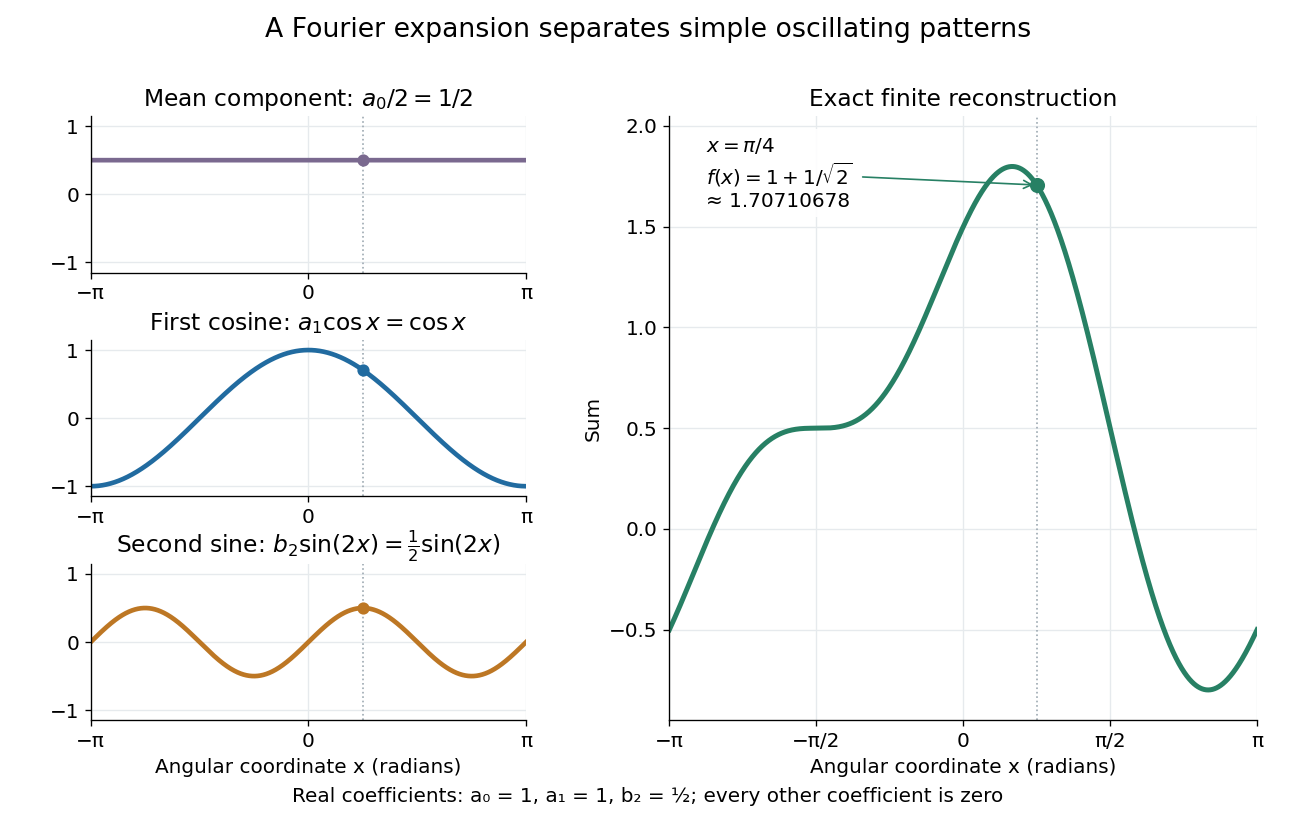
The change of viewpoint is useful because many linear problems act separately on these modes. The second derivative maps $\sin (nx)$ to $-n^2\sin (nx)$ and maps $\cos (nx)$ in the same way. Consequently a differential equation that is complicated for a whole profile can become a simpler calculation for each Fourier harmonic. A linear time-invariant system similarly has a separate response to each complex exponential. Superposition combines the responses when the relevant sums and operations are justified. ^[ref].

The infinite case contains a subtlety absent from the finite example. Under pointwise convergence of a piecewise smooth Fourier series, the value at a jump discontinuity is the average of the two one-sided limits. For a square-integrable function, the complex Fourier series instead converges in the $L^2$ norm: the integrated squared error tends to zero. Neither statement says that the error becomes small everywhere at once. A square wave shows the difference vividly through the Gibbs phenomenon.

A historical source for this connection between profiles and modes is Joseph Fourier's 1822 book Théorie analytique de la chaleur. Chapter III develops expansions in sines and cosines while studying the propagation of heat. The heat equation gives a continuing application of this approach. ^[ref].

The frequency response gives the change in complex amplitude of a sustained oscillation under a linear time-invariant system. If the impulse response is finite or has absolute summability, substituting $x[n]=e^{\mathrm{i}\omega n}$ into its discrete convolution yieldsThus $|H(\omega )|$ is the amplitude gain and its complex argument is the phase change. Real sinusoids follow by taking real or imaginary parts. Here $\omega$ is radians per sample; $\omega =2\pi f$ for $f$ cycles per sample. A physical sampling rate converts that normalized frequency into cycles per second.

For a trailing moving average,with removable singularities evaluated from the finite sum. In particular $H(0)=1$. For $M=5$ and $\omega =2\pi /5$, the five roots of unity sum to zero, so the oscillation is canceled. At small positive frequencies in the first pass region, the real sine ratio is positive and the phase factor gives a delay of $(M-1)/2$ samples.

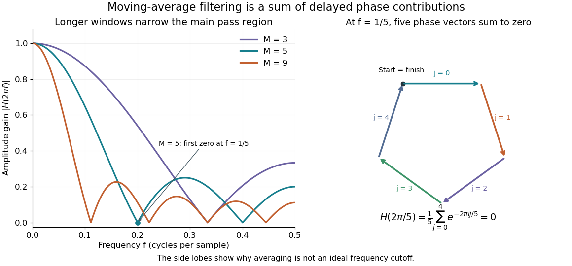
Increasing $M$ moves the first zero to $\omega =2\pi /M$, narrowing the main region of large gain. It does not create an ideal low-frequency cutoff: later side lobes transmit some higher-frequency components, and suppressing a component is only helpful when that component is unwanted. The frequency plot is the same operation as the delayed-sample average; the five-vector diagram explains one exact zero geometrically.

For a finite-dimensional continuous-time linear time-invariant system $\dot{x}=Ax+Bu$ on ${\mathbb{R}}^n$, with constant matrices $A,B$ over the real numbers, no state constraints, and every piecewise continuous function $u:[0,T]\to {\mathbb{R}}^m$ allowed as a control input without an amplitude bound, controllability in any fixed $T>0$ is equivalent to the controllability matrix having rank of a matrix $n$. The same equivalence holds with all square-integrable functions as inputs. A stronger useful statement iswhere $e^{AT}$ is a matrix exponential and $\mathrm{im}\mathcal{C}$ is the column space. Thus a rank of a matrix $r<n$ leaves only an $r$-dimensional affine subspace reachable at that time. ^[ref]

The Kalman rank criterion allows arbitrarily large commands as $T$ shrinks. It does not assert controllability with bounded control inputs, nor test a general nonlinear dynamical system just by counting its inputs. For the double integrator, $B=(0,1{)}^T$ and $AB=(1,0{)}^T$ give two independent directions, despite there being only one control input.

The Laplace transform is $\hat{f}(p)={\int }_0^{\infty }{e}^{-pt}f(t)dt$ and converts differentiation into multiplication by $p$ plus initial data.

A linear filter obeys the superposition principle: filtering $\alpha x+\beta z$ gives $\alpha T[x]+\beta T[z]$. Many familiar examples are also linear time-invariant systems, represented by an impulse response and convolution. Linearity alone does not imply time invariance: multiplying $x[n]$ by the index $n$ is linear but changes its behavior when the same input is shifted.

The moving average is a finite impulse response example implemented by arithmetic; a band-pass filter can instead be built from a series RLC circuit. Their frequency responses explain which oscillations pass through. Choosing a filter means choosing how much amplitude, timing and detail may change, not simply removing every visible fluctuation.

Reachability in control theory asks about a particular initial state $x_0$ and target $x_1$: does some admissible control input make $x(T)=x_1$ at the declared time $T$, or at some allowed duration? Controllability requires this for every pair in the declared state space. This is a property of state evolution, distinct from graph reachability.

For a linear time-invariant system, solving the ordinary differential equation by a matrix exponential givesThe first term is the unforced endpoint. Reachability in control theory asks whether the control input can supply exactly the displacement $x_1-e^{AT}{x}_0$. The timing matters because the same command is carried by different amounts of subsequent dynamics. ^[ref]

Here is a contrasting mathematical example with one shared control input:The controllability matrix has rank of a matrix one. Since $\frac{d}{dt}(z_1-z_2)=0$, the difference is invariant under every allowed control input. From $(0,0)$ the reachable set is the diagonal $z_1=z_2$ when input amplitudes are unrestricted: $(1,1)$ is reachable at $T=2$ using $u=1/2$, while $(1,0)$ is impossible at every duration. Having a control input appear in both state equations did not give independent control of both states. This reachable set is pictured alongside the bounded double integrator below.

Signal processing transforms or analyzes signals to extract information, change a representation, or improve a measurement. Examples include smoothing a sensor record, selecting a band of frequencies, and decomposing a recording through Fourier analysis. A signal is a mathematical representation of a physical record; deciding which variation is meaningful and which is noise is part of the problem.

A linear filter offers a simple entry point. Its output is assembled from weighted copies of its input. A moving average can reduce rapid variation, but it also changes timing and can erase useful detail. The worked example below makes that tradeoff explicit rather than treating a smoother plot as automatic improvement.

Two complementary views make the subject appealing. An impulse response describes the effect of a localized input; a frequency response describes the effect of a sustained oscillation. For a linear time-invariant system, both describe the same operation, connected by convolution and Fourier analysis. ^[ref].

A transfer function packages the response of a linear time-invariant system into a rule for turning a plant input into a plant output. Instead of solving a differential equation separately for every signal, take a Laplace transform, multiply by $G(s)$, then transform back. This also makes it possible to compare slow and fast oscillations through the continuous-time frequency response.

Here consider a continuous-time, causal, finite-dimensional linear time-invariant system with one plant input $u(t)$ and one plant output $y(t)$. With every initial state set to zero, its transfer function is defined byThe ratio $G(s)=Y(s)/U(s)$ is used where $U(s)\ne 0$ in a common Laplace convergence region; $G$ describes the system, independently of that particular plant input. Zero initial state matters: stored motion or another nonzero initial condition can contribute to the plant output even when the plant input vanishes. ^[ref]

The first-order low-pass filter below shows the same transfer function predicting both a step and a sustained sinusoid. Its pole gives a decay rate, its value at zero gives the eventual gain, and its values along the imaginary axis give the continuous-time frequency response. These descriptions make a useful bridge between a physical relaxation model and control theory calculations.