For a photon, . Using Planck constant , speed of light and givesThe Rayleigh criterion for a circular aperture of diameter is , set by the first zero of its Airy disk. Thus the ideal diffraction-limited resolution isThe conversion to transverse separation uses the small-angle approximation. An order-of-magnitude estimate instead gives and ; the distinction is the chosen resolution criterion. These are aperture limits, before instrumental aberrations and detector sampling.
Both the incoming and outgoing spherical wavefronts contribute to the path excess. At aperture radius , with axial distances before and after the aperture,The outer edge of the th Fresnel half-period zone has . HenceTherefore the outer radius is . The paraxial approximation is excellent because . Treating the illumination as a plane wave would incorrectly omit the source-side path curvature.
At normal incidence between lossless media with real positive acoustic impedances , continuity of pressure and normal particle velocity gives the pressure transmission amplitude . Since the mean acoustic intensity is , the fraction of incident energy transmitted isThis is acoustic reflection and transmission at an interface. With the supplied acoustic impedances,A thin water-based gel layer excludes air gaps and approximately matches the body's acoustic impedance. About of incident energy would otherwise reflect at the air-body interface. The coupling is also needed on the return journey, so it strongly improves the detectable echo. These figures concern interface transmission, before absorption within tissue; the gel is approximated by the stated water value.
Take nearest-neighbour separation , a common spring constant , and one scalar displacement per atom. For a monatomic chain, the harmonic approximation near a potential minimum, Newton's second law and a normal mode giveThe monatomic-chain dispersion relation has one acoustic phonon branch, with near the origin. The first Brillouin zone ends at , where and the group velocity vanishes.
For alternating masses , choose a two-atom cell of length . The coupled normal modes give the diatomic-chain dispersion relation with equal springs,The first Brillouin zone now ends at . The minus branch is the acoustic phonon branch; its two atoms move together at long wavelength. The plus branch is the optical phonon branch; at the atoms move oppositely with a stationary centre of mass and . For the edge frequencies are and , with a gap between them.
If , the two branches reduce to and , touching at . This is zone folding in an equal-mass diatomic chain: identical sites actually have a primitive unit cell of length . A doubled cell folds the monatomic branch but opens no gap. Equal masses alone do not specify all possible spring models; the sketches assume equal nearest-neighbour spring constants.
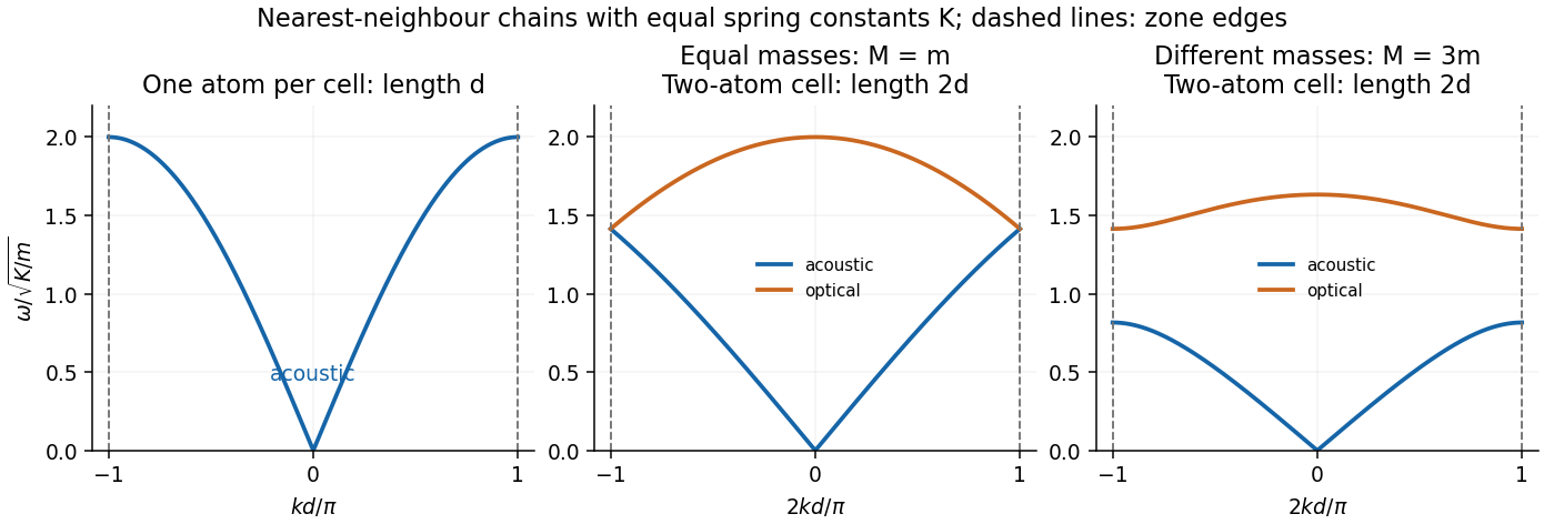
Monatomic and two-atom-chain dispersion relations, with explicitly chosen cell lengths and zone edges
. Details. Under the one-carrier Drude model, the magnitude of the Hall coefficient gives an effective carrier densityConvert the material mass density to and its molar mass to . The atomic number density isHere is the Avogadro constant. The positive Hall coefficient gives a hole-like response in a one-carrier interpretation. The Hall carrier count versus valence distinction matters: beryllium has two valence electrons, but the result is neither two free Electrons nor a literal fractional atom donating charge. Its energy bands and Fermi surface invalidate the simple isotropic one-carrier inference. Electron-like and hole-like contributions with different charge carrier mobilities can yield this sign and effective count.
Substituting into the damped harmonic oscillator equation givesFor nonnegative viscous damping, the cases areThe PDF's request to express these conditions in terms of is dimensionally inconsistent with its definition : already has units . With the unnormalised equation , the equivalent comparisons are , or . Also is the undamped natural angular frequency, not in general the driven displacement peak.
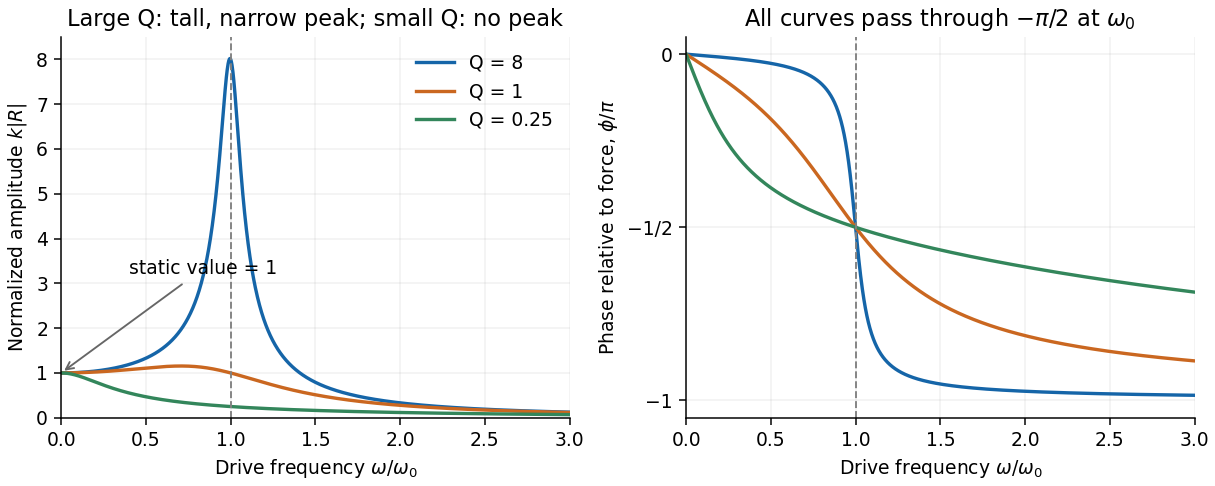
For the steady response of a forced harmonic oscillator, write and use the same complex amplitude convention for the driving force. Substitution givesThus the response magnitude and displacement phase relative to the force areThe phase goes from at low frequency, through at , towards at high frequency. The static magnitude is , while the high-frequency magnitude is approximately .
Define the quality factor by . If , the displacement peak occurs at ; for the magnitude decreases monotonically from its static value. For there is a tall narrow peak close to , of height approximately and width approximately . At very small the resonant peak disappears and the response is broad. The plotted functions are normalized as , at fixed .
The original diagram is a series RLC circuit, so the same electric current passes through all three elements. Choose capacitor electric charge positive on the plate into which positive enters. Kirchhoff's voltage law givesDividing by inductance givesThe correspondence to the forced harmonic oscillator is , , , and . The stored energy is ; its balance is , confirming the damping sign.
The capacitor-charge complex amplitude isFor fixed driving-voltage amplitude, maximizing minimizesDifferentiate:The positive-frequency minimum therefore hasThis is the resonance of charge, or capacitor voltage. If the stated inequality fails, their maximum is at zero frequency, and no positive displacement-resonance peak exists. The electric current has the additional factor , and instead peaks exactly at for every .
The precise bandwidth depends on the output: this is the distinction between displacement and current bandwidths of a series RLC circuit. For current output, or voltage across the resistor, the electrical impedance givesThe half-power points satisfy . Their positive roots areChanging capacitance shifts the centre without changing this absolute width. For the charge response in part (d), the exact half-height points instead obeywhen both exist their separation only approaches at large quality factor. Therefore the printed capacitance-independence claim is exact for current or resistor-voltage output and an approximation for the preceding charge resonance.
For a narrow band-pass filter, use current or resistor-voltage output and make small, counting source, load and inductor losses in the total electrical resistance. Increase ; if a specified centre frequency is to remain fixed, adjust with to keep fixed. Capacitor-voltage output alone is not a band-pass response because it has a nonzero DC limit.
In Fraunhofer diffraction, the relative propagation phase across the aperture is linear in aperture coordinates. If is its largest transverse size, the neglected quadratic path term must be small: for an observer at distance ,For a finite-distance point source a distance away, also require if the illumination is to be treated as a plane wave. Numerical factors depend on whether is a radius or full width and on the permitted phase error; the condition expresses a small Fresnel number.
One can place both source and screen sufficiently far away, or collimate a point source with a lens and observe the aperture in the back focal plane of a second lens. In the latter arrangement rays of each outgoing direction focus at one point, with ; the lens removes the need for a physically distant screen. A laser beam approximately uniform across the aperture can supply the incident plane wave. The sketches distinguish an actual far field from its focal-plane equivalent.
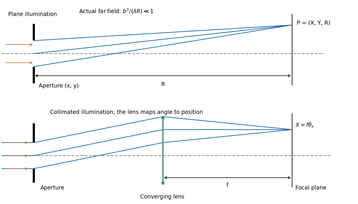
Let the aperture occupy the plane, with coordinates and opening . Write for the incident scalar complex amplitude and for its dimensionless amplitude transmission, including any imposed phase. The observation point has transverse coordinates , corresponding to the PDF's , and axial distance . Also is the wavenumber and .
The Huygens-Fresnel principle expresses the propagated field, up to common prefactors and an approximately constant obliquity factor, asIn the paraxial approximation, expand the path asThe last term is negligible in the Fraunhofer diffraction limit, while the first two terms and are common across the aperture. Factoring them out leavesIt is the two-dimensional Fourier transform of the transmitted aperture field, evaluated at transverse wavevector . For appreciable observation angles the corresponding exact directional components are used rather than .
Represent equal narrow slits at by two contributions with equal complex amplitudes. In a direction the path difference is , soTherefore double-slit interference givesThe bright interference fringes satisfy , with a central maximum. In the small-angle region,Dark fringes lie halfway between bright ones. Exactly, spacing is uniform in , not in at large angles. The first panel of the pattern figure below shows the narrow-slit result.
A relative phase changes the sign of one slit field. Their sum becomesThe central interference fringe is now dark. The maxima move to , while the minima occur at . Thus the pattern shifts by half a fringe, near the axis, but its angular fringe separation remains . This assumes the glass changes phase uniformly and introduces negligible absorption or beam deflection.
For a rectangular slit centred at , the one-dimensional Fraunhofer diffraction integral isThe two equal apertures have centres at ; the glass subtracts their fields. ThereforeThis is phase-reversed double-slit diffraction: the narrow-slit interference factor is multiplied by the single-slit diffraction envelope. In the limit , the normalized envelope tends to one, recovering part (d).
The interference minima and envelope minima obey, respectively,Near the axis these are and envelope zeros . Here , so every envelope zero already coincides with an interference minimum. The envelope strongly reduces the outer fringes; its central value is nonzero, but the total intensity still vanishes at because the two fields cancel. The sketch uses the small-angle coordinate; the equations above specify the exact angular zeros.
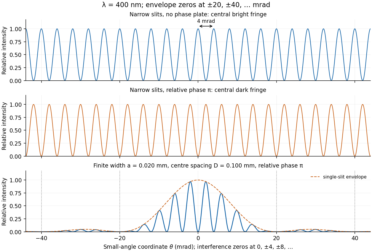
Unshifted and phase-reversed narrow-slit fringes, and the phase-reversed finite-width pattern with its envelope
. Details. In division of amplitude, one incident beam is split into two or more parts at a partially reflecting interface; they follow distinct paths and are recombined. The Michelson interferometer and thin-film interference use this principle. In division of wavefront, spatially distinct parts of the same wavefront are selected and allowed to overlap, as in double-slit interference. Both require adequate optical coherence; wavefront division particularly exposes the need for spatial optical coherence between the selected regions.
The beam splitter sends transmitted and reflected portions into perpendicular arms. Each mirror returns its beam to the splitter, where the two returning fields recombine towards the detector. A collimating lens provides approximately plane illumination. A compensating plate of the same glass thickness as the beam splitter can equalise the dispersive glass paths, which matters especially for broadband light.
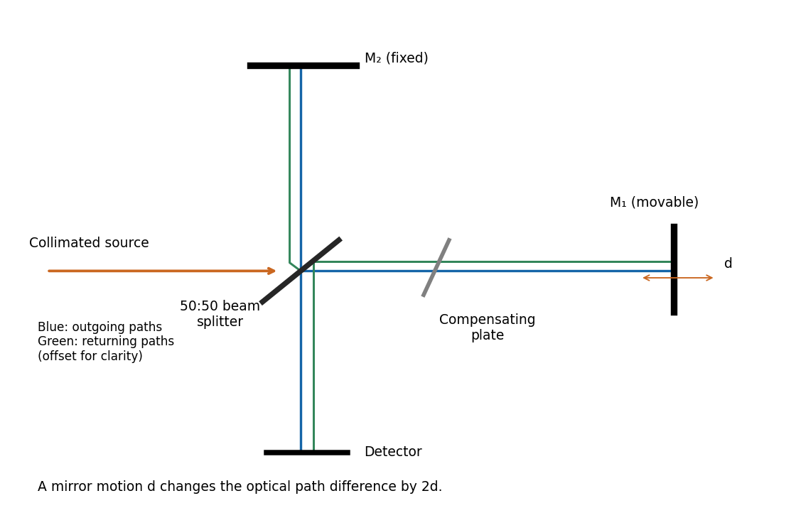
If the arm lengths are , the geometric optical path difference in air is , up to a chosen constant and any additional material paths. Moving one mirror by changes by . Fixed reflection phases can be absorbed into the reference position of a bright or dark fringe.
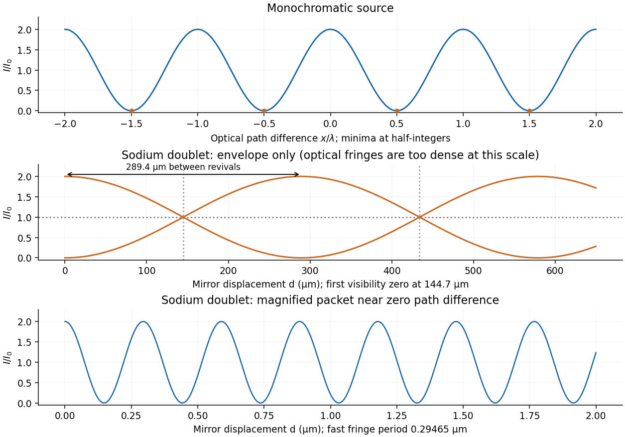
Take the two interfering complex amplitudes to have equal intensities and relative phase . The interference cross term then givesThus the mean intensity is , the maximum is , and the minima areThe optical path difference period is and the mirror-displacement period is . The assumed equal intensities refer to the two fields at the chosen output, with matching polarization of waves and full optical coherence. They set the normalization; they should not additionally be interpreted as all incident light entering that output port. A physical lossless Michelson interferometer has a complementary second output.
The two sodium lines are distinct optical frequencies, so their rapidly oscillating mutual cross terms average to zero at the detector. Assuming equal line strengths and negligible individual linewidths, add their separate interferograms. Write and . With the total mean output intensity,For mirror displacement this becomesThis is spectral doublet from Michelson visibility revivals. Since , . Numerically,The first interference visibility zero occurs at , with further zeros at odd multiples of that distance. Visibility is restored at integer multiples of . The signed envelope has period : alternate high-visibility packets have opposite fringe phase. Unequal line strengths leave a nonzero minimum visibility, and finite linewidths introduce a further decaying envelope; the wavelength data alone specify neither effect.


For mutually incoherent spectral components, the detected intensities add. If describes the mean output spectral intensity, the interferogram isSubtract the constant background, scan the mirror with a calibrated displacement, and take the Fourier transform with respect to delay . This is Fourier transform spectroscopy. The transform recovers the spectrum subject to detector response, finite scan length and any window function. Sampling the displacement finely enough to resolve the shortest optical fringes avoids aliasing.
Using the usual reciprocal-maximum-delay resolution estimate, , and , givesThe mirror displacement is measured from zero optical path difference. This delay-range resolution in Fourier transform spectroscopy is a conventional estimate: a specified window and resolution definition introduce a numerical factor. For example, a symmetric rectangular delay window has its first instrumental zero at , which would give under that particular criterion. The paper does not specify a line-profile criterion; the standard estimate states its convention explicitly.
The symbol here is linear mass density, with units . A short element has transverse forcebecause small slopes give . Its mass is . Applying Newton's second law, dividing by , and taking the limit gives the wave equation on a string,The derivation assumes constant positive tension, small transverse displacements and slopes, a flexible string with negligible bending stiffness, and negligible damping. Variations of tension due to the motion enter beyond the linear approximation.
A characteristic wave impedance relates an effort-like quantity to its conjugate flow-like quantity in a single travelling wave: for a mechanical wave these are force and velocity, and their product is power. The sign depends on the propagation and force conventions. Use the transverse force transmitted towards increasing , . A rightgoing travelling wave has transverse velocity , soThis is the positive characteristic impedance of a stretched string. A leftgoing component has with the same force orientation. Its units differ from pressure-based acoustic impedance because it uses force, rather than force per area.
For a rightgoing harmonic travelling wave in the lossless string, its force and transverse-velocity complex amplitudes satisfy with real . Thus the supplied mean-power expression giveswhere is the displacement complex amplitude and for convention . The same result follows directly from instantaneous string power averaged over a cycle. The amplitudes here are peak amplitudes; with root mean square force or velocity the factor is absent. If reflections return to the driver, its net mean input is still , but its input mechanical impedance need not equal the travelling-wave value .
At an ordinary point or a massless join, the string is continuous, soWith no concentrated transverse force or point mass, transverse force balance requiresFor the common tension in this problem, the slope is therefore continuous as well. A jump in linear mass density changes wave speed, but introduces no finite inertial force at a zero-length join. A point mass, external support force, or unequal tensions would require modified boundary conditions.
Place the join at , with an incident wave travelling from medium 1 towards medium 2. WriteContinuity of displacement and slope gives and . Hence reflection at a density step on a string givesFor , : the reflected transverse displacement has a phase reversal of . For , and there is no displacement-phase reversal. The transmitted displacement has no phase reversal for positive real mechanical impedances.
The reflected and transmitted mean-power fractions areFor strictly positive finite linear mass densities, ; a finite density step cannot produce exact total reflection. The ideal limits areThe first behaves as a fixed end; the second as a free end. In the free-end limit the transmitted displacement tends to , but its mechanical impedance tends to zero, so it carries vanishing power. Thus total reflected energy does not require a vanishing boundary displacement. “Entirely reflected” at a merely large density contrast is an approximation.
There is no reflected wave when the characteristic mechanical impedances match:for the same tension. Then , and . If tensions were independently adjustable, the general condition would be , together with transverse-force matching; equality of densities alone would no longer be the universal criterion.
Use the quantum free electron model: conduction Electrons move as independent particles in a three-dimensional box of volume , with a uniform positive background replacing the ionic lattice potential. Neglect the detailed periodic potential and explicit electron-electron interactions; the interior one-electron dispersion relation is . The boundary confines the particles, and its detailed shape does not affect the bulk state count in a sufficiently large sample.
The Electrons are spin- fermions: each spatial quantum state accommodates two opposite spin states, with occupations given by the Fermi-Dirac distribution and the Pauli exclusion principle. A fixed number of conduction Electrons and thermal equilibrium are assumed. Collisions can be represented by a phenomenological momentum relaxation time for transport, but are unnecessary for the equilibrium state counting here. These assumptions distinguish the quantum model from a classical Maxwell-Boltzmann Electron gas.
Impose periodic boundary conditions on a large cubic box. The allowed wavevectors occupy a lattice of cell volume in wavevector space. Including the two spin states, the number of states with magnitude at most isUsing and differentiating gives the total, spin-summed three-dimensional free-electron density of states,It counts states per unit energy; divide by for states per unit volume per unit energy. At zero temperature, the Fermi-Dirac distribution fills all states up to the Fermi energy, givingWriting givesThe energy zero is the bottom of the free-electron band. The electron Fermi temperature is .
The occupation probability of an individual one-electron state is the Fermi-Dirac distribution,At , it is a step: one below and zero above it. Heating rounds the step over an energy range of order a few , creating empty states below and occupied states above the chemical potential. At every positive temperature, .
For fixed in the three-dimensional free electron model, the chemical potential is determined by ; it is not exactly constant. In the degenerate regime , the Sommerfeld expansion givesIt is therefore reasonable in a simple low-temperature sketch to set , provided this approximation is stated. The figure includes the leading small shift. At much higher temperature the fixed- approximation fails and the distribution approaches the classical dilute limit. The plotted occupation is , rather than the energy distribution .
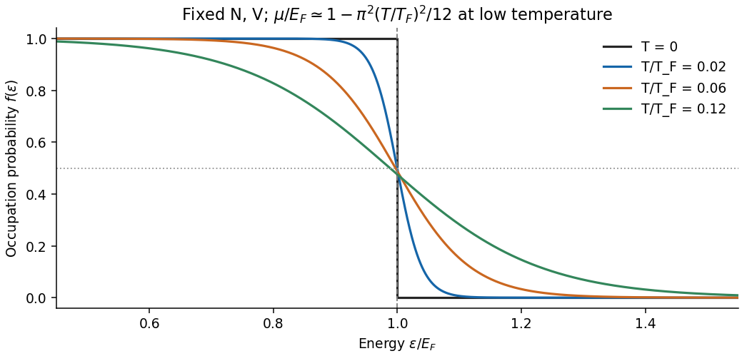
Thermal rounding of Fermi-Dirac occupations at fixed particle number, with the leading chemical-potential shift
. Details. 
Only a shell of energy width of order near the Fermi energy can change occupation: much lower states are blocked by the Pauli exclusion principle. The thermal-shell estimate of electronic heat capacity countsTo recover the rough coefficient requested in the paper, assign each of these active particles an excitation energy of order . ThenThe differentiation matters: the active shell itself widens as temperature rises. This argument explains the small linear-in- electronic heat capacity; its shell width and average excitation energy are heuristic, so it does not establish a precise numerical prefactor.
A controlled calculation from the Fermi-Dirac distribution gives a nearby but different result. At fixed particle number, the Sommerfeld expansion yieldsThus is a rough estimate of the exact free-electron coefficient , not an exact consequence of the stated density of states. Both require .
Assume sodium supplies one conduction Electron per atom. The supplied Fermi energy givesThe gas is strongly degenerate at room temperature. For one mole, and . Using the requested estimate,The supplied mass density determines the answer per unit volume: . ThereforeThe density is not needed for the molar heat capacity once is supplied. Using the precise Sommerfeld expansion coefficient instead gives .
Either electronic estimate is only about of the stated measured total. Most of the total heat capacity comes from lattice phonons, whose high-temperature Dulong-Petit law limit is . The remaining difference from need not be electronic: anharmonic lattice effects and the difference between heat capacity at constant pressure and heat capacity at constant volume also contribute. The paper does not specify the measurement constraint, so the two totals should not be equated exactly.
A Bloch state in a crystal experiences a periodic lattice potential. Its band dispersion relation encodes the lattice response, so an effective mass allows a wavepacket's acceleration under a weak applied force to be described without explicitly following the microscopic periodic forces.
In one dimension the wavepacket group velocity and semiclassical equation for crystal momentum areDifferentiating the first equation with respect to time givesDefining yieldsThis band effective mass is controlled by band curvature, not the slope. A band minimum has positive ; a band maximum has negative Electron and is often more conveniently described with positive-mass electron holes. In three dimensions the inverse effective mass is generally a tensor, . The scalar formula assumes motion along a specified direction in an isolated band, weak fields and negligible interband transitions; the bare Electron mass has not physically changed.
Let denote the elementary charge, so an Electron's charge is . In the relaxation-time Drude model with positive transport effective mass,The steady drift velocity is , defining positive electron mobility . The current density is opposite to the Electron drift:By the definition of electrical conductivity, , soIts units are . The mobility definition alone establishes the result in the scalar linear-response regime; the relaxation-time equation supplies a microscopic approximation for .
Interpret “3 mm wire” as a circular wire of diameter , and take the current density as uniform. One conduction Electron per atom givesUsing , the drift velocity corresponding to a current magnitude of isIt points opposite to conventional electric current. A simple distance scale over the cycle is , but this treats the magnitude as constant. For sinusoidal mains, alternating-current drift excursion gives zero net displacement after a full cycle.
If is the usual root mean square current, and the displacement amplitude and total absolute drift distance per cycle areIf instead denotes peak current, these become and . The paper does not state peak versus RMS; the characteristic drift is the boxed on whichever current convention is chosen. It also does not explicitly say diameter; taking as the radius would reduce all these velocities and drift distances by four. None of these distances is the microscopic path travelled at roughly the Fermi velocity between scattering events; that path cannot be obtained from the supplied current alone.
In a normal metal, the electrical resistivity can often be approximated using Matthiessen's rule,Static impurities, defects and grain boundaries scatter conduction Electrons even as , giving the residual resistivity. Thermal lattice phonons add a temperature-dependent contribution through electron-phonon scattering. In a clean three-dimensional acoustic model, small-angle electron-phonon transport at low temperature gives at low ; once thermal phonon populations are approximately classical, the resistivity is approximately linear in . An electron-electron contribution proportional to can be relevant in some low-temperature ranges.
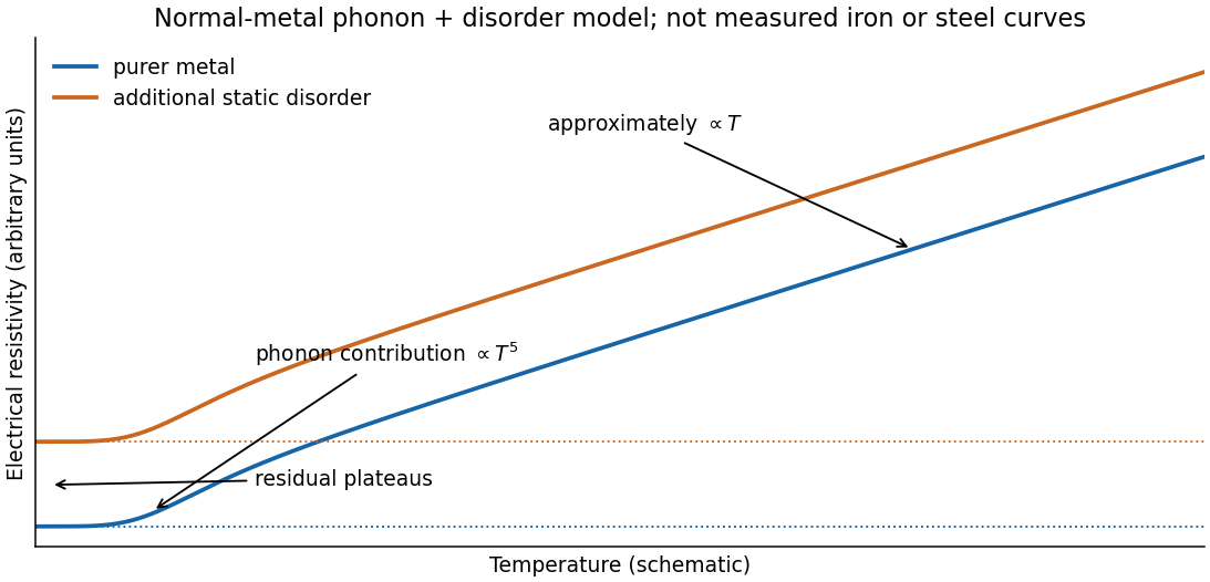
Schematic normal-metal resistivity with residual, low-temperature phonon and approximately linear high-temperature regimes
. Details. 
Carbon in mild steel, together with associated disorder, strain and microstructural changes, adds scattering and generally raises the residual resistivity relative to purer iron. Thus a dilute alloy may have a similar broad phonon-dependent rise but a larger baseline. The sketch is a generic phonon-plus-disorder model, not measured iron data. Iron's magnetic scattering and phase changes, and real steel's phases and processing history, can add structure; the simple sum is approximate rather than an exact material law. The expected explanation is greater Electron scattering from the added carbon and resulting disorder.
Doping changes the mobile carrier population by introducing controlled impurity levels. In an intrinsic semiconductor, the filled valence band is separated from the nearly empty conduction band by a band gap . Thermal excitation produces an electron-hole pair, so the Electron and hole number densities obey . A electron hole represents a missing valence-band Electron and behaves as a mobile positive charge carrier. For nondegenerate bands in thermal equilibrium,Here are the effective density of states, the band edges, and denotes the chemical potential, conventionally called the Fermi level. The semiconductor mass-action law holds in this nondegenerate equilibrium regime.
In a tetrahedrally bonded elemental semiconductor such as silicon, a substitutional group-V atom has an extra outer Electron relative to the host. It is a donor impurity: a shallow level just below can ionise, releasing an Electron to the conduction band and leaving a fixed positively charged donor. The resulting n-type semiconductor has Electrons as majority carriers and holes as minority carriers. Conversely a group-III substitution supplies one fewer bonding Electron. An acceptor impurity can take an Electron from the valence band, leaving a mobile electron hole and a fixed negative acceptor; the resulting p-type semiconductor has holes as majority carriers.
The impurity state is shallow because the Electron or hole responds to a screened Coulomb potential and an effective mass, rather than the bare atomic potential. A simple hydrogenic donor estimate iswhere is the relative permittivity. This is a useful scaling model, with real band anisotropy and central-cell effects omitted. Dopants are fixed in the lattice; their ionisation changes mobile carrier numbers without making a uniformly doped bulk sample carry a large net electric charge.
The charge neutrality condition isWhen shallow dopants are almost fully ionised and , an n-type region has and . A p-type region similarly has and . Thus compensation by the opposite impurity type reduces the majority-carrier density; the total dopant concentration is not generally the mobile carrier density. At sufficiently high impurity density the degenerate semiconductor regime requires the full Fermi-Dirac distribution and these exponential approximations fail.
There are three useful temperature regimes. At low temperature, dopant freeze-out leaves many shallow levels un-ionised. In the extrinsic regime, the dopants are largely ionised and set the majority-carrier density. At high enough temperature, intrinsic pair creation dominates and approach . The Fermi level moves towards the conduction band with donor doping and towards the valence band with acceptor doping. The electrical conductivity isDoping therefore controls conductivity and its carrier type, but ionised impurities also scatter carriers and can reduce charge carrier mobility. Carrier density and mobility must both be considered.
A p-n junction forms when p-type and n-type regions are joined within a semiconductor. Initially the concentration gradients drive diffusion current: Electrons diffuse from the n region to the p region and holes in the opposite direction. Recombination removes mobile majority carriers near the join, exposing fixed positive donors on the n side and fixed negative acceptors on the p side. This forms a depletion region and an electric field directed from n to p. Its drift current opposes diffusion. At equilibrium the net current vanishes and the Fermi level is uniform, although the band edges vary spatially through band bending.
For an abrupt nondegenerate junction with fully ionised dopants, its built-in potential isUnder the depletion approximation, the space-charge densities are on a p-side width and on an n-side width . Integrating Poisson equation and imposing zero field outside gives andMost of the depletion width therefore extends into the more lightly doped side. The schematic shows the impurity levels before contact and the resulting space charge and potential after contact; there is no externally extractable equilibrium battery voltage from the built-in field alone.
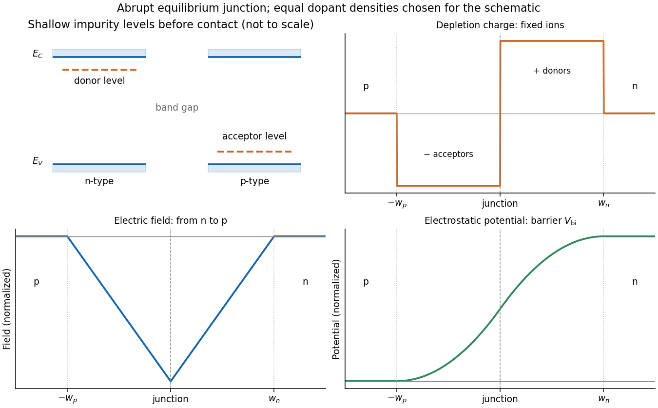
Shallow donor and acceptor levels, and charge, field and potential in an equilibrium abrupt p-n junction
. Details. 
A forward bias, with p positive relative to n, reduces the barrier from towards and injects minority carriers across the junction. In the ideal low-injection, diffusion-controlled regime this produces the Shockley diode equation, . Reverse bias increases the barrier and the depletion region; only a small thermally generated minority-carrier current flows before breakdown. Reverse-biased depletion regions also give a voltage-dependent junction capacitance. Real devices have recombination, leakage, series resistance and breakdown mechanisms beyond the ideal law. Controlled doping creates majority and minority carriers, and their junction produces a depletion barrier that makes rectification possible.
The convolution of two aperture functions in one dimension isWith Fourier transform convention , the convolution theorem statesThe first identity follows by substituting the convolution integral, putting , and separating the resulting double integral into times . For an absolutely integrable pair the interchange is justified by absolute convergence; finite optical apertures satisfy suitable integrability assumptions.
In Fraunhofer diffraction, the observed field is the Fourier transform of the transmitted complex aperture field. For two identical slits, let be one slit and use a pair of Dirac delta distributions to locate the centres:Consequently . For a rectangular slit, , giving a single-slit diffraction envelope times the double-slit interference factor in intensity. A phase reversal replaces the plus between the deltas by a minus, giving instead, as in B7.
More generally, an -slit array is a single-aperture function convolved with a finite comb. Its field contains the factorThis separates the narrow diffraction grating maxima from the individual-aperture envelope. The same reasoning holds in two transverse dimensions. Multiplying an existing aperture by an additional finite mask instead convolves their field transforms and can broaden features. These are operations on complex fields: intensity is the squared modulus of the final field and cannot generally be substituted into the field-level convolution theorem.
In thin-film interference, coherent beams reflected at the two faces of a transparent film overlap. Let the film have refractive index , thickness , and internal ray angle , determined by Snell's law. For vacuum wavelength , the propagation part of the relative phase isAlthough the internal round-trip ray length is , the two emergent rays must be compared on the same outgoing wavefront. Subtracting their external lateral path contribution gives the effective optical path difference , explaining the cosine rather than its reciprocal.
Reflection also changes phase. At normal incidence in lossless positive-index media, the electric-field Fresnel equations give : reflection towards higher index reverses sign, whereas reflection towards lower index does not. If the two interfering reflections differ by one such phase reversal, their total relative phase is modulo . Then reflected maxima and minima obeyIf there are zero or two reversals, the conditions interchange. These bright/dark conditions assume overlapping beams with adequate temporal optical coherence; complete cancellation further requires equal amplitudes. In transmitted light, a lossless complete film has complementary intensity variations because reflected plus transmitted power is conserved.
For multiple internal reflections at normal incidence, summing the geometric series gives the exact film reflection amplitudeThis includes both the amplitude mismatch and repeated-beam interference. A normal-incidence antireflection coating on substrate index can cancel reflection at one wavelength when and : both interface reflections reverse sign and the film's round-trip propagation adds , with equal interface amplitudes. A varying thickness or angle selects different maxima for different wavelengths, producing the colours of transparent films in white light. Broad bandwidth and large incidence angles generally prevent perfect cancellation across all wavelengths.
A dispersion relation specifies the allowed angular frequency of a wavevector . A single harmonic wave has constant-phase surfaces moving at the phase velocity,For two nearby components, use the identityThe slowly varying envelope moves at . Taking a narrowband limit gives the group velocity,More generally, expand around the central wavevector of a wavepacket. The linear term translates its envelope at ; the quadratic and higher terms produce group velocity dispersion and packet distortion. This interpretation needs a sufficiently narrow spectrum and weak enough absorption and distortion for an identifiable envelope to persist.
For light in a transparent material, , soThe derivative is evaluated at the wavepacket's central frequency and is the vacuum wavelength. In a nondispersive medium with constant , the two velocities coincide and a packet can propagate without dispersion. In normal optical dispersion , the displayed model gives .
The two velocities can differ even without material dispersion: a waveguide mode with has and , with . The phase velocity is not a signal speed. Near strongly absorbing resonances an anomalous derivative can also make the group velocity exceed or become negative; reshaping then prevents its simple identification with information transport. Relativistic causality constrains the signal front, not the speed of an arbitrary moving phase or distorted intensity maximum.
Articles by others on the same topic
There are currently no matching articles.