For the same massless spring of spring constant , Hooke's law gives the vertical simple harmonic motion about the displaced equilibrium position:Gravity shifts the equilibrium extension but does not change this frequency. Use the measured sample means in the ratio estimate. For small measurement errors, logarithmic differentiation givesAssuming the two frequency estimates have independent errors, their variances add. Writing for their common fractional standard uncertainty, monomial uncertainty propagation yieldsThis is a first-order uncertainty formula, rather than an exact identity for an arbitrary noisy ratio. It assumes that errors in the two measured frequencies have zero covariance.
There is a statistical distinction in the wording: the standard deviation of individual repetitions is not the standard error of their sample mean. If the supplied describes individual trials, the frequency means have errors , and the ratio formed from those means instead satisfiesThus the printed formula describes either a single-pair ratio or a convention in which already denotes the uncertainty of each averaged frequency. Under either consistent interpretation, independent repeated measurements reduce statistical error in proportion to . Halving it requires trials in total for each mass, or additional trials. Repetition alone does not reduce a fixed systematic error.
The spacecraft clock measures proper time , while a clock at rest with Earth measures the launch-to-emission interval . Neglect Earth's subsequent motion and gravity, as in the intended special relativity model. The Lorentz factor and time dilation giveIn Earth's inertial frame, the spacecraft's displacement at emission is . ThereforeHere and the speed of light is . The distance is evaluated at the emission event, using simultaneous Earth-frame endpoints, as required by relativity of simultaneity; the return signal has not yet reached Earth. A distance assigned on the spacecraft's simultaneous time slice is different: Earth has moved away at for in that frame, giving light-hours. Specifying the reference frame is essential to the numerical answer.
Use dimensions for mass, length and time. The reduced Planck constant, gravitational constant and speed of light have dimensionsFor to have the dimensions of a length, dimensional analysis requiresThe first equation gives ; the third gives . Substitution in the second gives . HenceWith , and , the Planck length isThe proposed monomial fixes the dimensionless prefactor to one; dimensional analysis on its own cannot select an arbitrary dimensionless multiplier.
First intensity minimum. In Fraunhofer diffraction, the path difference between adjacent slits is , so the relative wave phase is . Summing the equal complex amplitudes as a geometric series gives the diffraction grating interference factorThe central maximum has . Its nearest zero occurs at , where the denominator is nonzero. ThusThere is a symmetric first zero on each side of the incident direction. The narrow slits are treated as having a sufficiently broad single-slit diffraction envelope.
Wavelength resolution and the missing order specification. Adopt the Rayleigh criterion: the principal maximum of one wavelength lies at the adjacent minimum of the other in the same nonzero diffraction order . For and , those directions obeyConsequently the ideal resolving power of a diffraction grating is , givingThe usual first-order reading therefore gives . Zero diffraction order cannot separate the two wavelengths, because both central maxima coincide.
The paper does not specify which diffraction order is observed, so is not an order-independent minimum. In the ideal infinitely narrow-slit model, the largest usable order for this positive wavelength separation must satisfy . Since , this permits , giving the formal all-order resultThat pair meets the criterion at . Order of is at grazing incidence and the corresponding longer-wavelength peak cannot propagate. In a real device, finite slit width, weak high-order intensity and screen acceptance may prevent such an extreme order from being used; those data are absent. Thus the specified-order expression, and when first order is intended, are the defensible resolution answers under the stated criterion.
For a photon, the photon energy formula and the vacuum relation give . For an Electron, the de Broglie wavelength gives the same momentum magnitude , but the nonrelativistic kinetic energy is . Using , and ,Thus, to the precision of the wavelength,The electron answer is its kinetic energy, as required for the diffraction experiment; its relativistic energy would additionally include the approximately rest energy. Since , the nonrelativistic approximation is well justified. Equal wavelengths imply equal momenta, not equal energies for particles with different energy–momentum relations.
Put the charged sheet at and the grounded plates at . By symmetry the electric field points away from the positive sheet with equal magnitude in the two gaps. A Gaussian pillbox crossing the sheet givesThe plate boundary conditions fix their electric potentials to zero. For the charged sheet between grounded parallel plates, the central potential isWith vacuum permittivity , . An Electron has electric charge , so moving from a grounded plate to this positive potential decreases its potential energy by . Conservation of energy then givesThe unrounded value is , about . Either plate gives the same speed. The ideal calculation neglects the electron's disturbance of the prescribed field and image-force effects at its release point, consistently with treating it as a test particle.
Powered vertical flight. Take upward velocity as positive, and let be the downward exhaust speed relative to the rocket. During the rocket's mass changes by , and exhaust mass leaves with Earth-frame velocity . Compare the momentum of the rocket plus this newly expelled exhaust before and after the interval:Discard the second-order product . The result is , orThe positive rocket thrust is . Integrating with and gives the rocket equation with gravitational loss:Using for the rocket alone without the exhaust momentum flux would give the wrong equation for this open system.
Orbital speed under the stated gravity assumption. A circular orbit of radius requires centripetal acceleration . If the magnitude of gravitational acceleration is the stipulated constant even at the orbit,This treats gravity as centrally directed for the orbital calculation, while retaining its constant magnitude. The subsequent flat-surface approximation treats its direction as locally vertical.
Burnout height. During the unpowered projectile motion, horizontal velocity is constant. At the top of the trajectory the vertical component vanishes, so the horizontal component must equal the orbital speed . At burnout, therefore,These follow either by integrating or by the vertical work-energy theorem. Substituting the preceding constant- orbital result givesThe vertical component is initially positive, as required to reach the orbit after burnout.
Alternative inverse-square interpretation. A real Earth's exterior Newtonian gravitational field is not constant over a altitude change. If instead means the surface value , then Newton's law of universal gravitation gives andUsing this orbital speed but the paper's constant- flat projectile motion approximation for the coast would giveThis alternative changes the global constant-gravity assumption; it is not the same model as the result. An exact curved Kepler orbit coast would also abandon the prescribed flat trajectory. The printed assumptions support the constant-magnitude answers above, while the inverse-square values explain the different answer obtained from the usual physical Earth-orbit formula.
Directions. Choose along the horizontal spindle from the pivot to the disk, and vertically upward. With lever arm and weight , the torque about the pivot isClockwise precession viewed from above has . The relation therefore requires the spin angular momentum to point along , from the disk toward the pivot. The disk spins clockwise when viewed from its outer face looking along the spindle toward the pivot. Looking from the pivot reverses that apparent rotation. The right-hand rule fixes these signs unambiguously.
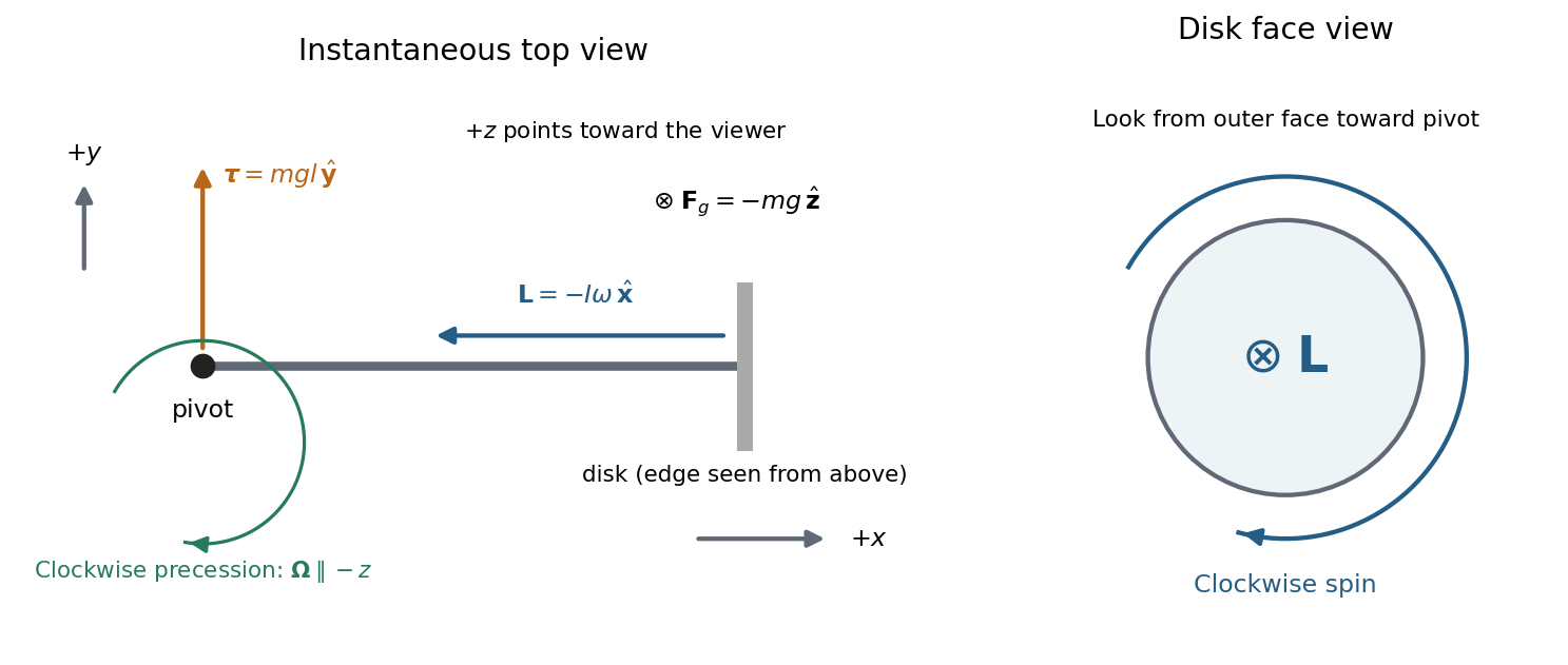

The drawing shows an instantaneous top view; the disk's angular momentum and the horizontal spindle turn clockwise together. The pivot force has zero torque about the pivot.
Rate of precession. For steady horizontal motion the spin contribution has magnitude and turns through in time . Its change is perpendicular to itself and has magnitude . HenceThis is the usual slow steady gyroscope precession relation. Any constant vertical angular momentum associated with steady precession has zero time derivative; the horizontal spin contribution supplies the changing component here. Transient nutation is excluded by the prescribed horizontal steady motion.
Clock design. Convert both rotation rates to angular frequencies:For the moment of inertia of a uniform disc, , so the mass cancels:
Spin friction. At fixed geometry, reducing increases . The precession period, , therefore decreases. This trend holds while slow steady precession remains a suitable description; it cannot be extrapolated to a stopped disk.
Counterweight. To oppose the disk's gravitational torque, place the counterweight on the other side of the pivot, at . The net torque isA horizontal axle can remain fixed when this vanishes, givingFor the fixed spin direction already found, counterbalanced gyroscope precession has signed rateMoving the counterweight outward from the pivot first slows the clockwise motion, eliminates its driving torque at balance, and then reverses the steady motion to counterclockwise. A counterweight on the disk's side would add to the gravitational torque. These statements neglect axial spin moment of inertia of the counterweight and assume the stated horizontal motion, without a separately imposed precession at balance.
Momentum identity. From the Lorentz factor, . The relativistic three-momentum therefore satisfiesTogether with relativistic energy , this gives the energy–momentum relation .
Parent in the laboratory. The rest energy is , while the total relativistic energy is . ConsequentlyIts momentum magnitude is .
Daughters in the zero-momentum frame. The centre-of-momentum frame is initially the parent's rest frame. Conservation of momentum gives . Equal daughter rest masses then imply equal relativistic energies. Conservation of relativistic energy givesTheir speeds are thereforeThe two velocities are opposite, and . Their total kinetic energy is .
Invariant of the complete system. Before the decay, in the centre-of-momentum frame,After the relativistic two-body decay,In the laboratory, four-momentum conservation fixes the summed daughter energy to and their summed momentum to the parent's . Thus the same calculation isThe invariant is formed after summing the daughter four-momenta; adding their separate squared rest energies would omit the relative-motion contribution to the invariant mass of the pair.
Axial moment of inertia. In the original diagram is the outer radius and the inner radius. For uniform mass density , a coaxial annulus of thickness has . Therefore the axial moment of inertia of a hollow cylinder isSince , factorizing the fourth-power difference givesFor a solid cylinder , giving . For a thin cylindrical shell with fixed mass and , . The latter limit agrees with every mass element being at radius .
Undamped rolling oscillations. Let be axle displacement from the spring equilibrium. Rolling without slipping imposes . The sum of translational and rotational kinetic energy isThe potential energy is . Differentiating in the absence of damping, or applying the force and torque equations below, givesFor the thin shell , the effective inertia is , and the angular frequency of the simple harmonic motion isStatic contact friction supplies the required torque but does no work when the contact point is instantaneously stationary.
Damped force balance. Take rightward force as positive and counterclockwise rotation as positive. Write for the signed static friction at the bottom contact. ThenEliminate and use :Here has units , so has units and units . The stated drag force is interpreted as acting through the axle, with no additional viscous torque. An oil bath could also exert such a torque physically, but its magnitude is not specified by this force-only model.
Light damping. Substitution of into the differential equation gives . In the underdamped regime ,Taking real linear combinations gives the general damped harmonic oscillator displacementThe constants are fixed by the initial displacement and velocity. For example, release from rest at gives and . Light damping means , in which case and the envelope decays slowly compared with an oscillation.
Complex impedance. In sinusoidal steady state write physical voltage and electric current as real parts of and . The electrical impedance is a ratio of phasors; its magnitude gives the voltage-to-current amplitude ratio and its argument gives their phase difference. It is measured in ohms.
For an ideal capacitor, and . Consequently , givingWith this time convention the voltage lags the electric current by .
Bridge output. The original diagram has and in parallel in the upper-left arm, and and in series in the lower-left arm. The point labelled is connected to the upper supply node. Set the lower supply node to zero, so . Assuming the measured output draws negligible electric current, the two voltage dividers giveTheir difference is thereforeThe reactive-arm electrical impedances are
Balance. Setting and cross-multiplying gives . For this Wien bridge,The right-hand side must be the real number . Equating imaginary and real parts givesPositive capacitances require . In the equal-component case and , this reduces to
Band-pass output and phase. Preserve the requested voltage polarity: . Since ,Put . The equal-component ratio is , so the Wien bridge band-pass response isAt finite positive frequency, its imaginary part vanishes exactly when . ThusThe magnitude is maximal there and tends to zero at both frequency extremes, as expected for a band-pass filter.
A convenient continuous, unwrapped wave phase isIt decreases from as , passes through at , and tends to as . A principal-value plot instead jumps from to at resonance; both represent the same phasor. Reversing the output to would shift the phase by and make the resonant ratio , but that is a different output polarity from the one printed.
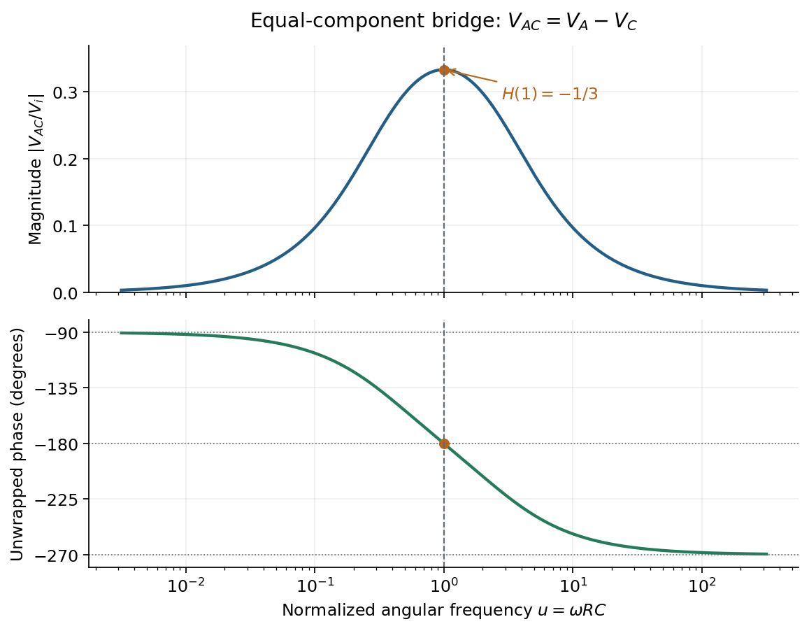
Band-pass magnitude and continuous phase for the printed output polarity VA minus VC
. Details. 
Reflection and central spot. At a boundary from lower to higher refractive index, the near-normal electric-field reflection coefficient is negative, . This gives a wave phase reversal on reflection from the glass plate through the air film. Reflection at the lens's glass-to-air underside has no such reversal. These are consequences of the Fresnel equations for the reflected electric field.
At ideal contact the film thickness is zero, so the two reflected contributions have zero geometrical optical path difference but a relative phase reversal. They produce destructive interference, and the central spot is dark. This conclusion concerns the film reflection; other lens surfaces can add a weak background.
Rings and their radii. At radial distance , let the air thickness be . The two relevant rays reflect at the upper and lower film interfaces. The lower reflection accumulates an extra round-trip optical path length , plus the relative reflection shift. As increases away from contact, alternating constructive and destructive thin-film interference forms Newton's rings. At near-normal incidence, a bright ring satisfiesThe extended source can illuminate these localized film fringes: each incident contribution interferes with its own two reflected paths; unrelated source points need not be mutually coherent.
For the spherical lens surface, geometry gives , so . Since , . Combining the equations yieldsThe bright ring is the first bright ring around the dark contact point.
Curvature from ring diameters. Writing , subtract the squared diameters to eliminate the unknown initial order:Using SI units,
Liquid-filled film. With film refractive index , still smaller than both glass indices, there remains exactly one relative reflection phase reversal. The round-trip optical path length is now , soHere is the illuminating vacuum wavelength, approximately its air value, rather than its shorter value inside the liquid. The ring labelled therefore has diameterFilling the gap contracts each ring radius by at fixed order and curvature.
Equation and interpretation. The supplied equation is the Time-independent Schrödinger equation for a nonrelativistic particle with mass in a prescribed potential energy . Equivalently,It is an eigenvalue problem for the Hamiltonian operator. A stationary energy state has full wavefunction . By the Born rule, is the probability of finding the particle in a small interval , with wavefunction normalization .
Infinite barriers. Infinite exterior potential energy excludes any finite-energy probability outside the interval. The infinite square well consequently has outside and the hard-wall boundary conditionsThe interior wavefunction must meet the zero exterior amplitude continuously. Its derivative need not be continuous across an infinite wall; imposing both zero value and zero derivative would eliminate every nonzero interior solution.
Ground state. Inside the well , so , with . Its general solution is . The left wall gives , and the right wall gives for . Thus the discrete energy eigenvalues are . The smallest, , is the ground state. Sinceits normalized wavefunction, choosing an irrelevant overall phase to make it positive inside, is
Finite barriers. For a finite step and constant particle mass, both and are continuous at . Wavefunction matching at a finite potential step follows by integrating the Schrödinger equation across a vanishingly small neighborhood of the step: a bounded potential cannot generate a finite jump in . The bound-state exterior solutions decay rather than vanish identically:Normalizability excludes the growing exterior exponentials. The equivalent interior boundary conditions are and ; neither boundary value is zero for the nontrivial ground state.
The ground state of a finite square well remains symmetric about and has no nodes. It bends smoothly into exponential tails at both walls, extending over a larger region than the infinite-well state. Its maximum after normalization is lower for the deep well considered here. When , the penetration length is short, so the two shapes are close except near the walls and in the exterior tails.
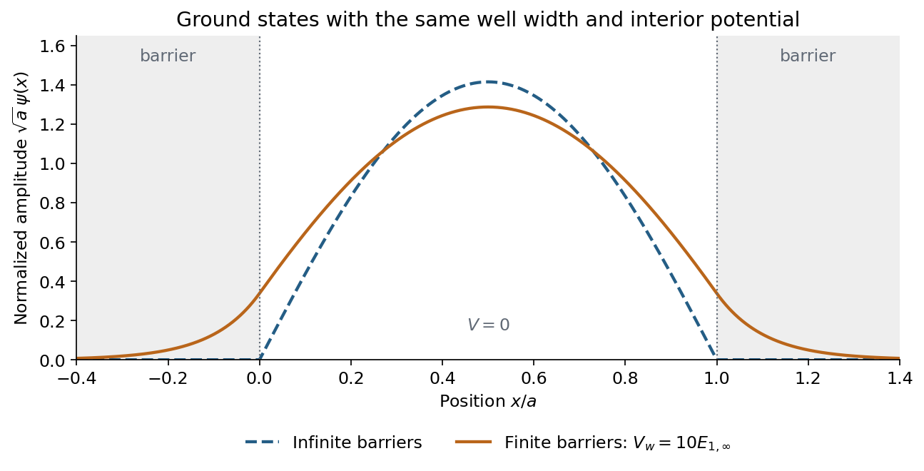
Normalized infinite- and finite-well ground states, with smooth exponentially decaying tails for the finite well
. Details. 
The finite curve is an illustrative exact matched solution with ; no numerical wall height is specified by the question.
Energy comparison. The finite barriers relax the confinement, allowing a less rapidly varying interior wavefunction and therefore smaller kinetic energy. More explicitly, the even interior solution is proportional to , and matching to the tails gives . The lowest root lies at , while the infinite well has . HenceAs , the tails disappear and the finite-well energy approaches the infinite-well value from below. This comparison uses the same zero of potential energy inside both wells.
Field of discrete masses. Newton's law of universal gravitation and superposition give the gravitational field away from the source points:It is the force per unit test mass, with units , and points toward each positive source mass.
Infinite circular cylindrical rod. Let be the radius of the circular cross-section, so , and write for the linear mass density. Choose a coaxial cylindrical Gaussian surface with radius and length . Translation and rotation symmetry make . The end caps have zero field flux because their normals are axial; on the curved surface the outward-normal component is the constant negative value . Gauss's law for gravity therefore givesThe gravitational field of an infinite uniform cylinder inside the material instead has enclosed mass , giving . The exterior result assumes a circular cylindrical rod; area by itself would not specify the exact near field of a noncircular cross-section.
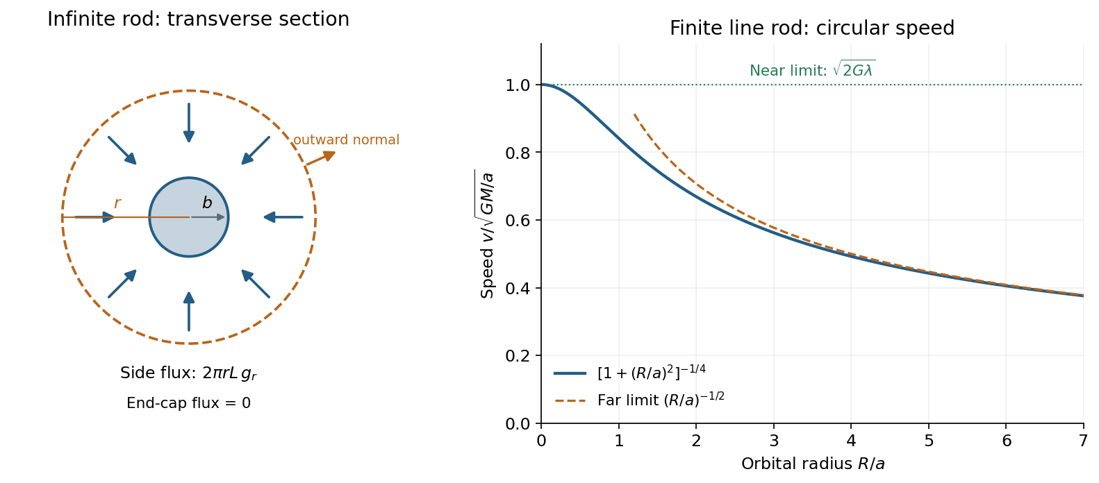
Gaussian-cylinder cross-section for an infinite rod and the circular-speed curve of a finite line rod
. Details. 
In the left panel the dashed circle is a transverse section of the coaxial Gaussian surface; the field points inward and the surface normals outward. Its side area is .
For an exterior circular orbit, Newton's second law equates the force required for centripetal acceleration to gravity:The orbital speed is independent of radius and of the orbiting object's mass, for orbits outside the infinite rod.
Finite rod. Taking the supplied field as the gravitational field of a finite uniform line segment, the corresponding balance at radius isSince , its two limits areThe first reproduces the infinite-rod result: a nearby observer sees a very long source. The second is the familiar circular orbit speed about a point mass, since a distant observer cannot resolve the rod's length. The dimensionless curve isIt starts at a constant plateau and decreases smoothly, approaching an dependence far away. For , , consistent with the sketch.
Derivation of the finite-rod field. Put the source along on the axis. In its central perpendicular plane, an element is at distance . Its field magnitude is , and its inward radial component has the extra factor . The axial components cancel between and . ThusReplacing by givesThe integral treats the source as a line mass. For a finite cylinder of nonzero cross-section, the displayed finite-rod formula is a thin-rod approximation, not an exact field for all . Its near-rod limit should therefore be read as , keeping the orbit outside the material; the apparent line-source singularity at does not describe the interior of a real cylinder.
An electric dipole is a localized pair of opposite electric charges, or more generally a neutral electric charge distribution with nonzero first electric moment. For charges and separated by displacement directed from negative to positive, the electric dipole moment isA neutral molecule can have a permanent electric dipole moment when its positive and negative charge centres do not coincide. An applied electric field can also produce an induced electric dipole moment by distorting an initially nonpolar electric charge distribution.
At distance in vacuum, expand the difference of the two point-charge potentials to first order in the separation. The leading electric potential isThe monopole term cancels because the net electric charge is zero. Taking gives the electric dipole fieldOn the dipole axis its magnitude is and its direction is along ; in the equatorial plane the magnitude is and the field points opposite to . The decay is faster than the field of an isolated point charge.
In a uniform external electric field, the opposite forces on the two charges cancel in their resultant but form a couple. Its torque isFor a fixed permanent electric dipole moment, the interaction potential energy isDifferentiating with respect to orientation recovers the torque. Parallel alignment minimizes and is stable against a small rotation; antiparallel alignment maximizes and is unstable. Rotating a fixed dipole slowly from parallel to antiparallel requires external work .
A nonuniform electrostatic electric field can also exert a net force. Expanding the two charge forces gives , which equals for a fixed dipole in a curl-free electrostatic field. Thus a suitably aligned dipole is attracted toward stronger field. An induced electric dipole moment requires care in computing energy: when for constant isotropic electric polarizability, building the dipole costs energy and the effective interaction is , rather than substituting directly into the fixed-dipole formula. These field, torque and energy effects explain molecular orientation and electric polarization.
A conservative vector field has path-independent work: the integral depends only on its endpoints. Equivalently, the line integral around every closed path in its domain vanishes. One can then define a single-valued potential energy byThe arbitrary additive constant in has no effect on the force. A useful zero is often chosen at infinity for a localized attractive interaction.
A differentiable conservative force has because the curl of a gradient vanishes. Conversely, a smooth curl-free field on a simply connected domain admits a global scalar potential. The domain condition matters: on the punctured plane, has zero curl away from the missing origin but closed-loop work around it. It is not globally conservative there. The existence of a local potential does not establish a single-valued potential throughout a domain with holes.
The work-energy theorem gives for kinetic energy . If all forces are conservative and has no explicit time dependence, thenThis is conservation of mechanical energy. In one dimension, an equilibrium occurs at ; a local minimum with is stable, while a maximum with is unstable. Expanding about a minimum gives , producing simple harmonic motion with .
Examples include the spring force with , the near-surface gravitational force with , and the central Newtonian gravitational field with . An electrostatic force on a fixed electric charge has , where is the electric potential.
Sliding friction provides a contrasting physical test: traversing a closed path still dissipates mechanical energy, since the frictional force opposes the local motion on both outward and return legs. Its work depends on path length and cannot be represented by a position-only . Total energy can remain conserved when the resulting internal energy is included. Also, even if at each instant, explicit time dependence gives ; a static conservative-field argument alone does not guarantee constant mechanical energy in that situation.
Faraday's law of induction relates an induced electromotive force to the rate of change of magnetic flux. Choose a positive orientation around a loop and its associated surface normal by the right-hand rule. For a stationary conducting loop,Unlike an electrostatic field, the induced electric field generally has nonzero curl; the differential form is . For a moving circuit, magnetic flux transport for a moving circuit includes the magnetic Lorentz force on the charges:where is the local wire velocity. Thus changing the field or moving a conductor can produce induction.
The minus sign is Lenz's law: an induced electric current, when a closed conducting path permits it, produces a magnetic field opposing the change of linked flux. It need not oppose the original field itself. For example, increasing flux through a loop produces a current tending to reduce that increase; decreasing the same flux reverses the current. The opposition is consistent with conservation of energy: external mechanical or electrical work is needed to maintain a change against its inductive reaction.
For a coil of turns, define the magnetic flux linkage , reducing to when every turn links the same flux. For fixed geometry and a linear magnetic response, self-inductance is defined by , and the coil's induced electromotive force isThe corresponding terminal voltage drop, with the passive sign convention, is . It opposes changes in electric current; it does not require the current itself to vanish.
Building the current from zero requires power . Integrating gives the energy stored by an ideal inductor:This energy is stored in the magnetic field and can be returned when the current falls. In a series RL circuit driven by a constant voltage , Kirchhoff's voltage law gives . Starting with zero current, , with time constant . This makes the resistance to rapid current changes directly observable. Two coils also have mutual inductance: changing primary current induces secondary electromotive force with a polarity determined by the chosen winding orientations, the principle behind a transformer.
For a light test particle of mass outside a spherical source of mass , Newton's law of universal gravitation gives . It is a central force, so its torque about the source vanishes and angular momentum is conserved. The motion therefore lies in a fixed plane when . Its gravitational potential energy is , and conservation of mechanical energy givesHere is specific orbital energy and is specific angular momentum. A Kepler orbit has polar equationThe angle is measured from periapsis. The conic section is an ellipse for and , a parabola for and , and a hyperbola for and . The circle is the elliptical case. The special case is radial motion and must be handled as a degenerate limit. Bound ellipses have the source at one focus, which is Kepler's first law.
For a bound orbit of semi-major axis , . Combining this with the energy equation gives the vis-viva equation:The particle therefore moves faster near periapsis and slower near apoapsis. Conservation of angular momentum also gives constant areal velocity, , expressing Kepler's second law. Using the ellipse's area and gives the orbital periodwhich is Kepler's third law.
A circular orbit follows from centripetal acceleration , giving and . The minimum escape velocity from radius follows from the marginally unbound condition :These ideal orbits neglect drag force, other gravitating bodies and changes in the central source. For two comparable masses, the relative two-body problem uses instead of . An orbiting object is continuously in free fall; the inward gravitational force changes its direction even when its speed is constant. These inverse-square results assume the physical variation of gravity with radius, rather than extending a near-surface constant- approximation to an entire orbit.
Articles by others on the same topic
There are currently no matching articles.