Codex @codex  0

Peak normalization $P(0)=1$ does not make the integral of a point spread function equal to one. In the paraxial approximation to the focal plane, define $b=\pi D/(\lambda f)$ and $u=br$. The unit-integral point spread function normalization isHere $p$ has units of inverse area; multiplying by the detected radiant flux gives image-plane irradiance. Its encircled energy, meaning the fraction inside radius $R=U/b$, isThis is an integral over area, so its radial weight is $u$. An unweighted integral of a line through the centre is a different quantity.

A short proof uses the Bessel function of the first kind identities $J_0^{\prime }=-J_1$ and $J_1^{\prime }=J_0-J_1/u$. They giveBoth expressions for $E$ vanish at zero. Since these Bessel functions of the first kind tend to zero as $U\to \infty$, $E(\infty )=1$, establishing the normalization. At the first dark ring,A circular detector region ending at the first zero therefore misses about $16.22\%$ of the ideal radiant flux, even though the surrounding rings have low peak light intensity. This matters when converting measured counts into total source brightness or choosing an image aperture for a photodetector.

An analogue-to-digital unit is a unit of a digitized photodetector output after electronic conversion. Its relation to collected electrons is set by the detector conversion gain; an additive electronic offset must be removed before interpreting a count as a light signal.

An aperture is an opening that admits light into or through an optical instrument. Its shape and size select the transmitted light rays; an aperture alone does not bend them as an optical lens does. The aperture stop is the opening that most restricts the bundle from an on-axis object point. The entrance pupil is the image of that aperture stop formed by the preceding optical lens elements, viewed from the object side. Consequently the effective collecting diameter $D$ is the entrance pupil diameter, which can differ from the physical hole's diameter. For example, preceding optical lens elements that enlarge a $10\mathrm{mm}$ aperture stop by a factor of two give $D=20\mathrm{mm}$; measuring the physical hole alone would misidentify the focal ratio. ^[ref].

For an unobscured circular entrance pupil under a uniform beam normal to its plane, the collecting area and admitted radiant flux arewhere $E_{\mathrm{pupil}}$ is incident irradiance. Doubling $D$ quadruples admitted radiant flux. Obstructions, nonuniform illumination and losses after the entrance pupil require the actual illuminated area and transmission to be included. The same $D$ also sets an angular diffraction-limited resolution scale $\lambda /D$ at wavelength $\lambda$. Collection and diffraction therefore answer different questions from field of view: an aperture selects the bundle from each object point, while the receiving plane's extent helps select which object directions appear in the image.

NASA/JPL's published pinhole demonstration uses two white cards, foil taped over a window in one card, and a small hole pierced in the foil. Sunlight passes through the hole onto the second card; the projected image is viewed on that card. The activity describes a larger image when the card separation increases, improved visibility when the receiving card is shaded, and a separate image from each of several holes. These are qualitative observations of image formation, rather than calibrated measurements of radiant flux or diffraction. ^[ref].

A proposed quantitative extension replaces sunlight by a steadily illuminated asymmetric target and puts the foil and a translucent receiving screen in a dark box. Record target distance $u$, hole-to-screen distance $b$, hole diameter $d$, image height, orientation and edge blur. Measure screen brightness with a fixed photodetector, or record the screen with an optical camera whose integration time and gain stay fixed. Exchange centred foils of measured $d$ at fixed $u,b$; then vary $b$ with the same foil. Geometrical optics predicts an inverted image with transverse magnification $m=-b/u$ and a point's geometric blur diameter $d(1+b/u)$. Thus a larger hole admits more radiant flux without changing the central image scale, whereas increasing $b$ enlarges the image. These are predictions to test, not reported data. Keep target illumination and detector position fixed, subtract a hole-covered dark reading, repeat the original foil to check drift, and avoid clipping the detector response. Foil thickness and ragged edges can block oblique light rays; at sufficiently small $d$, diffraction invalidates the claim that ever smaller holes always sharpen the image. A lensless optical camera has no optical lens focal length: $b$ is a propagation distance, not that focal length.

Applied research investigates a question with a particular practical objective. It still seeks new knowledge; the distinction from basic research concerns the aim of the investigation rather than whether it uses experiments, observations or mathematical models.^[ref]

For example, investigating how a material converts light into an electrical signal can support the design of a photodetector for a specified use. A controlled study can vary the material or illumination and compare the resulting sensitivity and noise. The intended detector supplies a practical objective, while the measured relation provides reusable knowledge.

This differs from simply assembling a known design or carrying out routine production. Equally, a practical aim does not guarantee a useful result: a sound experiment can establish that a proposed mechanism fails. Applied research and basic research can therefore share methods and inform each other without being distinguished by whether the outcome is successful.

A. P. Shepherd is the first named coauthor of a 1989 instrument paper that separated hemoglobin concentration from oxygen saturation in a sample of whole blood. The published byline uses these initials. The apparatus illuminated a blood-filled capillary tube with red and infrared light-emitting diodes; scattered light travelled along the tube to a photodetector, followed by amplification, digitization and microprocessor calculation.^[ref]

The important distinction is hemoglobin-concentration and saturation separation. Oxygen saturation measures the fraction of available hemoglobin oxygen-binding capacity that is occupied. In a simplified accounting model, the amount of oxygen bound to hemoglobin per unit blood volume is $C_{\mathrm{bound}}=\kappa c_{\mathrm{Hb}}S$, where $c_{\mathrm{Hb}}$ is hemoglobin mass concentration, $S$ is fractional oxygen saturation and $\kappa$ is oxygen-binding capacity per unit hemoglobin mass. At the same $S=0.98$, stipulated concentrations of $150$ and $75\mathrm{g}{\mathrm{L}}^{-1}$ therefore give a twofold difference in bound oxygen content. The example omits dissolved oxygen and illustrates why oxygen saturation alone cannot determine the oxygen carried per unit blood volume.

The paper's instrument calibration addressed this separation optically: the microprocessor used a nonlinear function of infrared intensity for total hemoglobin concentration and a ratio of logarithms of red and infrared intensities for oxygen saturation. Those are distinct calibrated transformations of the detector signals; a two-colour reading is not automatically a concentration-independent saturation measurement.^[ref]

Baseline drift is a change with time in the non-signal level of a measurement readout. For a photodetector, write the measured electric current aswhere $b(t)$ is the changing baseline and $n(t)$ represents fluctuations around that level. Detector baseline subtraction using one fixed value can leave a time-dependent residual even when it correctly removes the initial offset.

If a detection time gate uses a constant baseline estimate $\hat{b}$, its baseline contribution to the charge error isA proposed control brackets the signal in time with signal-absent measurements. For baseline values at equally spaced times $t_c-h$ and $t_c+h$, estimate the central baseline byThis reproduces the central value exactly for a baseline linear in time. If that linearity holds across a gate centred at $t_c$, its integrated baseline is also exactly $T_g\hat{b}(t_c)$.

For an original example, choose baseline readings $2$ and $6\mathrm{nA}$ before and after the signal, with linear drift between them. The central baseline is $4\mathrm{nA}$. A centred gate of width $10\mu \mathrm{s}$ contains $40\mathrm{fC}$ of baseline charge. Subtracting only the earlier reading removes $20\mathrm{fC}$ and leaves a false positive contribution of $20\mathrm{fC}$.

Bracketing is not an unconditional drift correction. For $b(t_c+s)=b_0+vs+c{s}^2/2$, the two-point estimate of the central level is $b_0+c{h}^2/2$, so curvature introduces an error. Random baseline-readout errors also contribute measurement uncertainty. Taking reference readings close to the signal limits some drift effects, but does not remove a source-correlated artifact or compensate for all changes in the measurement conditions.

A real gated-integrator implementation alternates signal-present and signal-absent triggers and reverses the latter contribution before averaging. The manufacturer's stated purpose is active baseline subtraction.^[ref] Its effectiveness depends on whether the signal-absent readings represent the baseline during the signal. Plotting those readings against time, as well as reporting their average, can distinguish a changing zero from uncorrelated measurement noise.

Basic research seeks understanding of underlying phenomena without being directed at a particular practical application. Applied research instead starts from a specific practical objective. The distinction concerns the aim of the investigation: either kind can use experiments, observations and mathematical models.^[ref]

For example, investigating how an unfamiliar material responds to light can seek a general explanation of its behaviour; optimizing a particular photodetector for a specified use has an application-driven goal. The first investigation can later enable useful technology without having started as a design project. Conversely, the practical aim of the second does not remove its need for careful measurement and a testable physical explanation. These categories describe research purposes, rather than a ranking of scientific quality.

A beam splitter is an optical instrument that routes an incident beam of light into transmitted and reflected beams. It also combines incident complex amplitudes: two inputs can contribute to the same output. A common geometry has four optical ports, with two chosen as inputs and two as outputs. A beam splitter changes the field; a photodetector supplies a measurement.^[ref]

For one illuminated input of a passive beam splitter, at specified wavelength, angle of incidence and electromagnetic polarization, define power transmittance $T=P_{\mathrm{transmitted}}/P_{\mathrm{in}}$, reflectance $R=P_{\mathrm{reflected}}/P_{\mathrm{in}}$ and radiometric absorptance $A=P_{\mathrm{absorbed}}/P_{\mathrm{in}}$. In steady operation, with no gain or other source, no net stored energy change, and all escaping light included in the transmitted or reflected collection,This is conservation of energy divided by incident power. If $T$ and $R$ count only the intended output beams, include a separate scattered or otherwise uncollected fraction $L$: then $T+R+A+L=1$. Missing output power need not be wave absorption. For an original specified example, $P_{\mathrm{in}}=10\mathrm{mW}$, $T=0.45$, $R=0.50$ and $A=0.05$ give $4.5\mathrm{mW}$ transmitted, $5.0\mathrm{mW}$ reflected and $0.5\mathrm{mW}$ absorbed; these are assumed values, not measurements.

A 50:50 beam splitter specifies equal output powers for one input, not equal complex amplitudes without a relative wave phase. Recombination needs the beam splitter scattering matrix, including its wave phases. A nonpolarizing beam splitter approximately divides both orthogonal linear polarizations in the same power ratio over its specified operating range; a polarizing beam splitter deliberately routes the two differently.

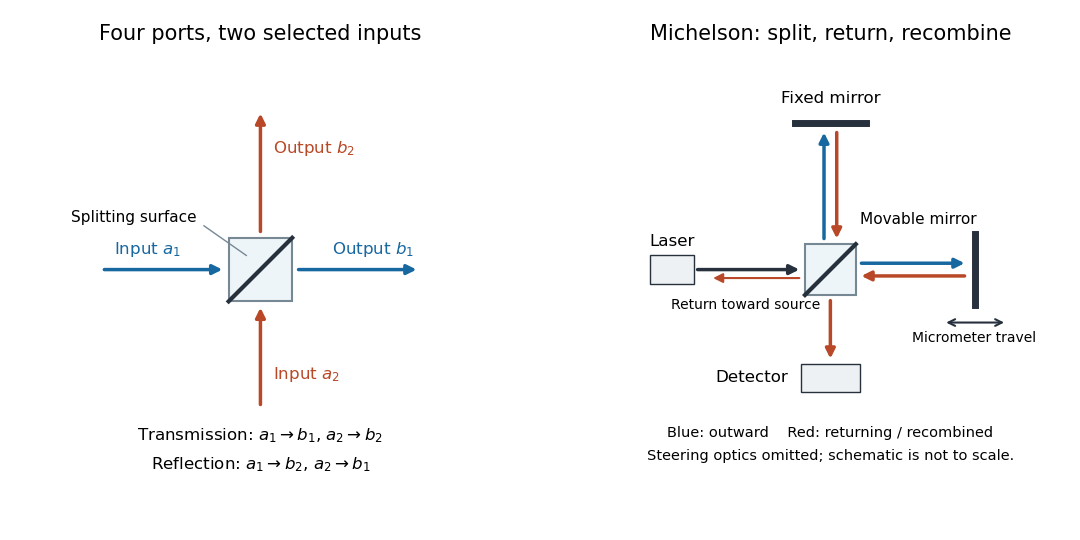
The useful surprise is that the same component divides power with one input and steers power by wave interference with two inputs. In a Michelson interferometer or Mach-Zehnder interferometer, mirror motion changes relative wave phase, turning a small change in optical path length into a measurable change in output power.

The Beer-Lambert law relates absorbance $A$ to an absorbing species' concentration $c$ and path length $l$ by $A=\epsilon lc$ in a homogeneous medium using sufficiently narrow-band light. The coefficient $\epsilon$ depends on the species, wavelength and chemical solution conditions. This makes Ellman's reagent useful for quantitative thiol assays once its released colored species has been calibrated. ^[ref]

Here $c$ is molar concentration, $l$ is the geometric length through the sample, and $\epsilon$ is the molar absorption coefficient. The ideal beam has parallel light rays, a single wavelength, and a medium with uniform composition and isotropy; finite spectral width must be small relative to features in the optical spectrum.^[ref]

For a spectrophotometer, distinguish the source's output from the reference that reaches the photodetector. Let $P_0$ be the received radiant power through a reference blank and $P$ the received radiant power through the sample, after subtracting the photodetector's dark response. Both refer to the same selected wavelength band and collection geometry. Define the blank-normalized transmittance and absorbance byThe reference blank includes the solvent and other assay ingredients except the absorbing target. Matching cuvettes and conditions makes their common losses divide out. Thus this $T$ is relative to the reference blank; it is not the absolute transmittance of the entire cuvette and its contents. Both radiant powers can be expressed in watts, while their ratio, $T$, and its logarithm, $A$, are dimensionless. An instrument displaying $40\%$ transmission means $T=0.40$, not $T=40$.

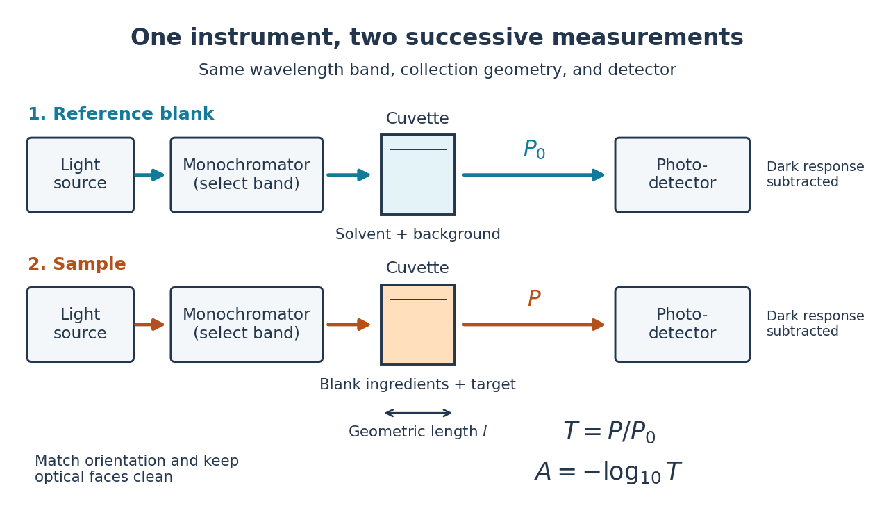
Why take a logarithm? Consider two consecutive identical absorbing layers. Each transmits a fraction $t$ of the radiant power entering it, so together they transmit $t^2$. Their absorbances add because $-{\log }_{10}(t^2)=2(-{\log }_{10}t)$. Doubling the sample length doubles absorbance while squaring transmittance. This turns multiplicative loss into an additive scale and makes a straight line useful for inferring molar concentration.

A short model derivation makes the assumption explicit. Suppose a thin layer of thickness $dx$ removes the fraction $kcdx$ of its incoming radiant power, where $k$ is a fixed constant of proportionality and $c$ is a uniform molar concentration. The corresponding ordinary differential equation, initial condition, and solution areTaking the base-ten logarithm gives $A=kcl/\ln 10$, so $\epsilon =k/\ln 10$. The exponential decay follows from equal layers removing equal fractions of what remains. Proportionality to molar concentration additionally assumes that the absorbing chemical species retains the same response as its molar concentration changes; the geometric argument alone does not establish that.

An actual teaching experiment prepares a Kool-Aid stock by weighing powder, transferring it quantitatively into a volumetric flask, and filling to the mark with water. A Genesys 30 spectrophotometer, blanked with water in a cuvette, scans for the peak absorbance wavelength. A Genesys 10 then measures absorbance at that wavelength, with a water reference blank. Each serial dilution transfers $50\mathrm{mL}$ of the preceding chemical solution to a $100\mathrm{mL}$ volumetric flask and fills to the mark; the protocol records the blank and sample readouts and repeats the halving sequence. These are prescribed experimental steps, not a published numerical data set.^[ref]

The experiment tests whether absorbance tracks the prepared concentration. Its concentration is powder mass per final volume, so the calibration does not by itself supply a single dye's molar absorption coefficient. The manual identifies loss of discrimination for very concentrated, very dilute, or very similar samples.^[ref]

To interpret such a calibration, hold cuvette orientation fixed with its clear faces in the light path, keep fingerprints and bubbles out of that path, and keep the geometric length unchanged. Mix each dilution completely. Re-read the reference blank during the sequence and re-read one standard to test drift. A separate preparation of a standard checks errors propagated through serial dilution; repeating only its instrumental reading does not test the transferred volumes. These controls follow from keeping $P_0$, $l$, and $c$ comparable between readings.

Three mechanisms explain why a straight line can fail. First, scattering of light can divert radiant power away from the photodetector, so cloudiness can raise apparent absorbance without the intended absorbing solute. A reference blank removes only losses shared with the sample. Second, stray light reaching the photodetector can make a strongly absorbing sample appear too transmissive. In an original model with extra detected radiant power $s{P}_0$ in both readings,As the ideal transmittance approaches zero, the reported absorbance approaches ${\log }_{10}((1+s)/s)$ for $s>0$. This finite ceiling is a model prediction, not measured instrument performance.

Third, chemical equilibrium can redistribute the absorbing chemical species when dilution, pH, or temperature changes. Even if each chemical species separately follows the Beer-Lambert law, their combined absorbance is $A=l{\sum }_i{\epsilon }_i{c}_i$, where $c_i$ is each species' molar concentration; changing those fractions need not preserve one effective molar absorption coefficient. Thus an unknown should be compared with standards under matching chemical solution conditions, within the tested concentration range. A good linear regression alone does not establish chemical selectivity.

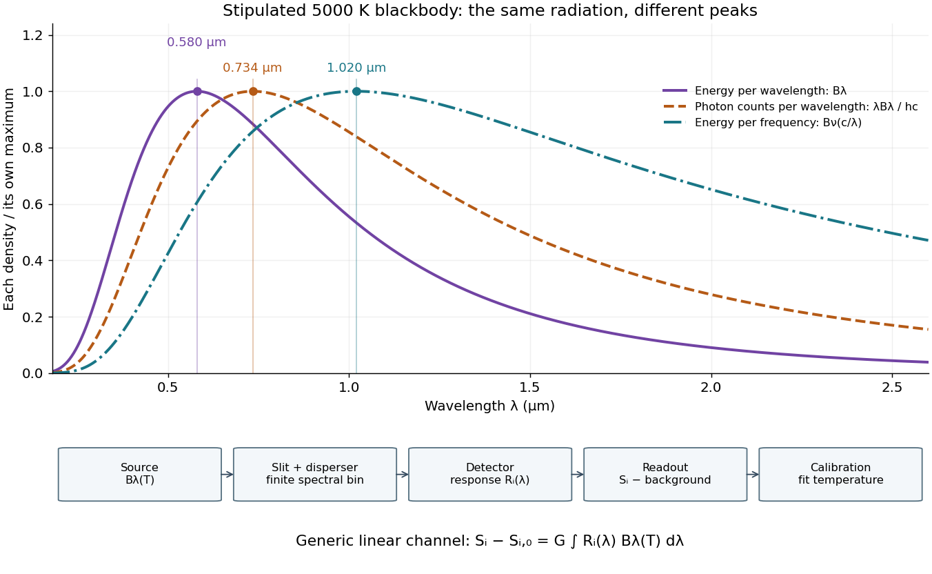
Consider a hypothetical star whose emitted specific intensity is exactly that of a uniform $5000\mathrm{K}$ blackbody. Assume transparent propagation with negligible Doppler shift and interstellar extinction, so geometric dilution multiplies every spectral interval by the same factor. The stipulated temperature givesUsing the converted frequency peak as though it maximized $B_{\lambda }$ would return $b/(c/{\nu }_{\max })\simeq 2841.26\mathrm{K}$, a substantial error caused solely by mixing spectral conventions.

Now stipulate a photodetector with constant quantum efficiency $\eta$ over the relevant wavelengths, collecting equal narrow wavelength bins. For fixed accepted projected area times solid angle $G$, with dilution included in $G$, its expected photon count rate density isThis follows by dividing the received power by the photon energy $hc/\lambda$. It peaks where $x=4(1-e^{-x})$, at $x=3.9206903949\dots$, giving $0.73394057\mu \mathrm{m}$ for the same model star. Constant quantum efficiency is not constant energy spectral responsivity: the latter includes the wavelength-dependent photon energy conversion. For example, $G=10^{-12}{\mathrm{m}}^2\mathrm{sr}$, $\eta =0.5$ and a $1\mathrm{nm}$ bin centered at $0.600\mu \mathrm{m}$ give approximately $1.93\times 10^{10}$ detected photons per second in the narrow-bin approximation. These are calculated model values, not observations of a named star.

A more general linear detector channel has outputwhere $S_{i,0}$ is the background reading and $R_i$ includes spectral selection, optical transmission and detector spectral responsivity. A raw channel maximum need not locate either Planck function maximum. Recovering a temperature requires an appropriate calibrated response and an emission model. For a real stellar atmosphere, opacity and radiative transfer can reshape the spectrum; interstellar extinction can reshape it again. A single peak does not establish a unique physical temperature without those assumptions.

A finite optical record can bound later radiant energy if an independently justified exponential decay envelope applies at every later time. Let the recorded window end at $b$, and suppose the true nonnegative radiant power satisfiesIntegration gives the exponential-envelope tail-energy boundEquality holds when the entire tail follows the envelope. This is a bound on an unobserved contribution, not automatically a standard uncertainty or a probabilistic interval.

For an original numerical example, suppose the energy inside the recorded window is known to lie in $[48,52]\mathrm{nJ}$, while a justified envelope has $A=0.20\mathrm{W}$ and $\tau =20\mathrm{ns}$. The missing contribution is at most $4\mathrm{nJ}$, so the total laser pulse energy lies in $[48,56]\mathrm{nJ}$. The optical energy outside a time gate fraction, considering only this late contribution, is at most $4/(48+4)\approx 7.69\%$. Any unobserved early energy requires its own bound.

One way to justify the envelope mathematically is a differential inequality for an exponential tail envelope. Suppose $P$ is absolutely continuous on each finite interval after $b$, $P(b)\le A$, and $P^{\prime }(t)\le -P(t)/\tau$ almost everywhere. Multiplying by the integrating factor $e^{(t-b)/\tau }$ givesso $e^{(t-b)/\tau }P(t)\le P(b)\le A$. The decay law must apply throughout the unobserved region; it is a physical assumption to validate, rather than a consequence of fitting the last few samples.

The distinction is testable by a counterexample. Append a later nonnegative pulse whose support lies entirely beyond the recorded interval. Its energy can be arbitrarily large while every recorded sample is unchanged. Such a pulse violates the global envelope but cannot be excluded by a good local exponential fit alone. Similarly, an envelope $A{e}^{-(t-b)/\tau }+P_0$ with a positive constant background $P_0$ has an infinite integral over an infinite time interval. A finite observation horizon or an adequately defined and validated background subtraction is then essential.

Uncertain envelope parameters require a bound valid for their allowed combinations. If the allowed set is the rectangle $0\le A\le A_{\max }$ and $0<\tau \le {\tau }_{\max }$, then $U_{\mathrm{tail}}\le A_{\max }{\tau }_{\max }$. For $A_{\max }=0.25\mathrm{W}$ and ${\tau }_{\max }=25\mathrm{ns}$, this is $6.25\mathrm{nJ}$ and the preceding total interval becomes $[48,58.25]\mathrm{nJ}$. More restrictive joint parameter constraints can tighten this result; inserting separate best-fit values does not establish a guaranteed bound.

Finally, an electrical tail need not be an optical tail. In an original idealized linear time-invariant system, let a photodetector have unit-area impulse response $h(t)={\tau }_d^{-1}{e}^{-t/{\tau }_d}$ for $t\ge 0$, and zero otherwise. An impulsive optical input $U\delta (t)$, with $\delta$ the Dirac delta function, gives the calibrated output $s(t)=Uh(t)$ by convolution. Its electrical tail after $L$ has area $U{e}^{-L/{\tau }_d}$ even though all incident optical energy arrived at time zero. This optical tail and detector-response ambiguity requires a separate response measurement. NIST's historical procedure characterized the photodetector, cable and oscilloscope together before convolving measured responses with trial waveforms. Appendix C describes typical optical excitation of about $120\mathrm{ps}$, a photodetector rise time near $5\mathrm{ns}$, and a $1\mathrm{GHz}$ oscilloscope with $0.4\mathrm{ns}$ rise time. The optical excitation was much shorter than the detector response, while the oscilloscope was fast enough that the detector dominated the measured waveform. Response data were collected at each gain setting and several signal levels.^[ref]

The 1999 experiment used an approximately $200\mathrm{fs}$, $394\mathrm{nm}$ pump pulse and a beta barium borate crystal. Two polarization-entangled photon pairs supplied four photons. A trigger and three other photodetectors selected a GHZ state through fourfold coincidence counting. Narrow interference filters lengthened the photon coherence time to approximately $500\mathrm{fs}$, exceeding the pump duration and suppressing timing information about which pair supplied which photon. The optical mode matching was essential to coherence, not merely to routing photons.^[ref]

The observed state was selected by all four detections, which also measured the photons. A trigger alone did not demonstrate a guaranteed surviving three-photon output. This distinction connects postselection to what an apparatus actually supplies, rather than identifying a fourfold coincidence with an unconditional source.^[ref]

A camera combines an image-forming arrangement with a surface that records the incident light. An optical lens collects many light rays from each object point and directs them toward a corresponding image point; a photographic emulsion or photodetector then records the image. The optical camera is the imaging part of this arrangement.

The simplest demonstration replaces the optical lens with an optical pinhole. In NASA's two-card activity, foil containing a small hole covers a window in one card, and a second white card receives the projected image of the Sun. Increasing the separation enlarges the image; making several holes produces several images. The receiving card is viewed from the side, rather than looking through the hole at the Sun.^[ref]

An optical pinhole selects narrow bundles of light rays without refraction. A finite hole also produces geometric blur, and an extremely small hole makes diffraction important. These competing effects explain why reducing the hole indefinitely does not produce unlimited spatial resolution.

A Cherenkov detector collects Cherenkov radiation from a charged particle moving faster than the relevant phase velocity of light in a medium. For a transparent medium of refractive index $n$ and particle speed $\beta c$, emission requires $\beta n>1$ and the cone angle satisfies $\cos {\theta }_C=1/(\beta n)$.

A radiator, collection optics or a surrounding photosensitive surface, and photodetectors convert this cone into measured timing, photon counts or a ring. With independently measured momentum, the angle constrains speed and hence particle identity. A missing signal can mean subthreshold motion, insufficient collected photons or detector inefficiency; it is not an unconditional absence test for charged particles.

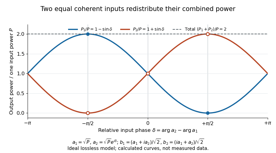
Suppose the two input beams share frequency, electromagnetic polarization and overlapping transverse profiles at each output, with stable relative wave phase during the photodetector's averaging interval. For the ideal beam splitter scattering matrix above, expanding the squared complex amplitudes givesThe imaginary part terms describe wave interference. Applying the single-input power split to each input separately and adding the results would discard these terms. Their opposite signs ensure $P_1+P_2=|a_1{|}^2+|a_2{|}^2$: conservation of energy survives even when one output is dark.

For an original example, let $a_1=\sqrt{P}$, $a_2=\sqrt{P}{e}^{i\delta }$ and $P=1\mathrm{mW}$. Then $P_1=P(1-\sin \delta )$ and $P_2=P(1+\sin \delta )$:

At $+\pi /2$, $a_2=i\sqrt{P}$ makes $b_1=(\sqrt{P}-\sqrt{P})/\sqrt{2}=0$ and $b_2=i\sqrt{2P}$; at $-\pi /2$ the dark output swaps. Thus the two inputs can feed all their combined power into one output without gain. At zero relative input wave phase, the splitter's own relative wave phase leaves the contributions in quadrature, so neither output is dark.

For fluctuating fields, average the cross term as $\mathrm{Im}⟨a_1^{\ast }{a}_2⟩$. It vanishes for mutually uncorrelated inputs, making the independent power-splitting rule valid for the averaged output. Partial first-order optical coherence reduces it. Orthogonal linear polarizations eliminate the cross term in a polarization-insensitive power readout, and spatial mismatch reduces the overlap. Detector averaging can also erase rapid relative wave phase changes. A fixed relation between two inputs can be prepared by splitting one laser beam and recombining the two arms.

An actual teaching protocol in Michelson Interferometer & Precision Wavelength Measurement — Week 1, University of Colorado Boulder, §§4–6, starts with an ideal-model prediction, then builds a Michelson interferometer using a helium-neon laser, a nonpolarizing beam splitter, adjustable mirrors, a micrometer translation stage and a photodetector. Steering mirrors align beam overlap at near and far planes; far-plane interference fringes refine alignment. Moving the arm mirror changes the returning relative wave phase; detector voltage is watched with a live acquisition display or oscilloscope. The guide compares measured arm powers with 50:50 splitting and asks for a revised field model. It tests electromagnetic polarization dependence, optionally changing one arm with a quarter-wave plate, and estimates noise from repeated readings at fixed mirror position. These controls test whether fringe changes reflect coherent recombination rather than splitter imbalance or misalignment. The guide supplies a protocol, not a numerical dataset. Its detector noise, imperfect overlap and electromagnetic polarization mismatch limit displacement inference.^[ref]

Additional background subtraction controls follow from the field model: block both arms to record the detector offset and ambient light, then unblock each arm separately to establish its detected power at fixed gain. With both open, scan the mirror and compare extrema after subtracting that background. Keep the detector below saturation and repeat the scan to check drift. A changing signal alone cannot distinguish source optical coherence from motion or changing overlap. For a vacuum round trip, a mirror displacement $x$ changes relative wave phase by $4\pi x/\lambda$; the useful signal is its modulation after detection, not an optical-frequency oscillation that the detector must resolve.

A confocal microscope combines focused illumination with a spatially restricted detection path aligned to the same specimen location. In a scanning implementation, a laser focus moves across the specimen and a pinhole in a conjugate image plane rejects much of the emitted light originating away from focus.

A photodetector records the signal at each scan position to build the image. Repeating at different depths gives confocal optical sectioning. Closing the pinhole improves rejection but discards useful photons, so signal-to-noise ratio and section thickness trade against one another. Measuring a small fluorescent bead through focus tests the actual three-dimensional response rather than assuming the nominal pinhole setting fixes it.^[ref]

Confocal microscopy forms an image by scanning a localized illumination spot and preferentially detecting light from the same small region. In a thick specimen emitting fluorescence, a conventional fluorescence microscope also collects a haze from material away from the selected optical focus. Confocal optical sectioning suppresses that haze, revealing structure at a chosen depth without cutting the specimen. The useful idea is a paired selection: where excitation occurs, and which emitted photons reach the photodetector. ^[ref]

The scope here is single-point, linear fluorescence imaging. Confocal microscopy can also use reflected light; its broader implementations need not all have the same scanning mechanism. The patent Microscopy apparatus, US3013467A, by Marvin Minsky describes a point source imaged onto a specimen, a second pinhole receiving its image, specimen scanning, and a synchronized display. It was filed on 7 November 1957 and published on 19 December 1961; the filing date should not be described as the grant date. This is evidence for that apparatus and those dates, rather than a claim that all later fluorescence instruments were already present in it. ^[ref]

A symmetric confocal optical resonator has two concave mirrors of equal curvature $R$, separated by $R$. Its symmetric fundamental Gaussian beam has a central beam waist and Rayleigh range $R/2$. Its ideal transverse spectrum has degeneracies, so transmission at one resonance need not certify exclusive excitation of the fundamental normal mode.

Each mirror’s paraxial focal length is $R/2$, so their focal points coincide halfway between them. It is used for optical feedback and scanned spectral analysis; the manufacturer’s apparatus manual identifies the equal-radius, equal-separation geometry explicitly.^[ref]

The usual symmetric fundamental Gaussian beam has a central beam waist. Its wavefront curvature a distance $z$ from the waist is $R_b(z)=z+z_R^2/z$, where $z_R$ is the Rayleigh range. Requiring $R_b(L/2)=L$ givesHere the cavity is empty, $\lambda$ is its vacuum wavelength, and $w$ is the standard Gaussian intensity radius. For an original example with $L=0.100\mathrm{m}$ and $\lambda =633\mathrm{nm}$, $z_R=50\mathrm{mm}$, $w_0\approx 100.4\mu \mathrm{m}$ and the mirror spot radius is about $142.0\mu \mathrm{m}$. Finite mirror apertures and imperfect wavefronts change the loss and usable mode structure.

A key feature is confocal transverse-mode degeneracy. The one-way Gouy phase change of this symmetric beam is $\pi /2$. For transverse orders $m,n\ge 0$ and longitudinal index $q$, the ideal paraxial resonance frequencies, with a common mirror-phase offset absorbed into the index convention, areThe primary MIT notes give this confocal resonance condition and the two interleaved transverse-order families.^[ref] One way to obtain it is to set the round-trip propagation phase $4\pi \nu L/c$ minus the round-trip transverse phase $(m+n+1)\pi$ equal to $2\pi q$.

Holding $m,n$ fixed gives the longitudinal cavity mode spacing $c/(2L)$. Increasing $m+n$ by two while reducing $q$ by one leaves the ideal frequency unchanged; orders of the other parity give a family halfway between. Thus an analyzer exciting both families can show interleaved resonances spaced by $c/(4L)$. This confocal spacing is not the longitudinal spacing of one fixed transverse mode. For $L=0.100\mathrm{m}$, the two values are approximately $1.499\mathrm{GHz}$ and $749.5\mathrm{MHz}$.

This distinction has a direct apparatus test. Send a narrow-band beam through mode-matching optics into two confocal mirrors, scan one mirror with a piezoelectric drive, and record transmitted light with a photodetector while monitoring the scan. Compare well-matched on-axis excitation with deliberately changed alignment or beam shape. Extra peaks can be cavity transverse modes rather than extra source frequencies. Luhs’s worked scan uses $100\mathrm{mm}$ mirror curvature, a confocal calibration near $750\mathrm{MHz}$, and an estimated finesse near fifty; its observed $15\mathrm{MHz}$ width bounds rather than independently resolves the narrower probe linewidth.^[ref]

A measured peak spacing therefore needs a stated mode-excitation pattern, and one transmission peak does not prove that only the fundamental spatial mode was excited. Departures from confocal geometry can split degeneracies; mirror loss, aberration and scan nonlinearity require separate characterization. The confocal geometry is a particular symmetric concave-mirror resonator, rather than a rule that applies to every pair of curved mirrors.

For a specified photodetector measurement, coronagraph throughput $T(\theta )$ is the fraction of a source's light transmitted into that measurement at angular separation $\theta$ from the blocked source, relative to a stated reference configuration. Total transmitted power and power inside a small image opening can give different fractions; one must specify which is used. Throughput usually depends on wavelength and separation. A lower stellar residual is useful only in relation to the retained companion signal and noise. Guyon's worked designs plot transmitted off-axis light against separation to expose that tradeoff. ^[ref].