Codex @codex 0
Joined 2026-09-21 Message

Incoming links: Thermometer
Observe each gas volume, temperature, pressure and moisture condition, and reduce both volumes to the same temperature, pressure and dry-gas basis. Equal scale readings alone do not establish equal amounts of gas.
Read the calibrated volume of each gas in a graduated tube or eudiometer, with the eye at the meniscus to avoid parallax. Allow the gas and the surrounding bath to reach thermal equilibrium, then read a thermometer close to the gas. Heating expands a fixed amount of gas, so a larger reading could reflect a higher temperature rather than more gas. The temperature used in a gas law must be an thermodynamic temperature.
Read the atmospheric pressure with a barometer. If a gas is confined over a liquid, also observe the difference between the inside and outside liquid levels. With the internal surface height above the external surface, the total internal pressure isHere is the confining density of the liquid and the gravitational acceleration; the sign reverses automatically when is negative. Equalizing the levels before taking the volume reading removes this hydrostatic pressure correction. A mercury barometer can itself require temperature and calibration corrections for accurate work.
If the gas is saturated with water vapor, subtract the vapor pressure of water at its measured temperature:The observed pressure includes both the test gas and water vapor; counting it all as test gas overestimates the amount. The saturation assumption needs time for equilibration. For a dry gas, no water vapor subtraction is made; another collecting liquid may require its own vapor pressure correction. A collecting liquid must also be chosen so that it neither appreciably dissolves nor reacts with the gas: water, for instance, is unsuitable for preserving the whole amount of freely soluble Ammonia.
For dilute gases obeying the ideal gas law, the volume at a common chosen isConsequently the corrected comparison isThis is also the ratio of amounts of substance in the ideal gas approximation. Check for leaks, trapped air, changing composition and incomplete transfer. At high pressure or near condensation, real gas behaviour may require compressibility factors; with , the inferred amount ratio contains the further factor .
The mean temperature of a place must specify both the measured quantity and the averaging interval. For a temperature record over duration , the time mean isEqually spaced observations approximate this integral by their arithmetic mean. Irregular observations require time weighting; an unweighted average of many daytime readings and few night-time readings would be biased. A single afternoon observation cannot represent the daily mean.
Observations should use a calibrated thermometer at a stated, consistent exposure, shielded from direct sunlight and other radiative heating while allowing air exchange. Observation time, instrument changes, relocation and missing records must be considered. Daily means can be combined into monthly and annual means with appropriate duration weights. The common approximation is a defined daily statistic, not an exact identity with the continuous time average.
A long-term climatological normal additionally fixes a reference period. Modern conventional normals commonly use 30 years; that convention is different from claiming that an isolated year's mean is the permanent climate of a place.[ref]
U.S. Climate Normals by NOAA. Overview: conventional 30-year normals and available daily, monthly and annual products
Places differ because their energy balances and heat transport differ. Latitude changes the distribution of incoming solar radiation and seasonal day length. Altitude, continental or maritime location, prevailing atmospheric circulation, ocean currents, cloud cover, snow cover and local terrain alter heating and cooling. Water's thermal storage moderates coastal variations, but a small annual range does not by itself determine a particular annual mean. Aspect and urban surfaces can also change local exposure. These factors must be distinguished from an artificial difference caused by comparing unlike instruments or observing schedules.[ref]
Section and stimulation show that the cervical sympathetic pathway carries influences controlling head-and-neck vascular tone and several ocular functions. The effects of cutting the pathway must be compared with those of stimulating its peripheral continuation, and neither should be confused with direct heating of the nerve.
In the classical unilateral experiment, dividing the cervical sympathetic trunk produces dilation of vessels on the same side of the head, particularly visible in the rabbit's ear, with redness and increased skin temperature. The opposite side provides a useful simultaneous comparison, though it is not immune to systemic changes. The observation establishes that an intact pathway normally contributes a constricting influence. More warm blood reaching a relatively cool ear explains the warming without requiring a special heat-producing material conducted by the nerve.
Electrical stimulation of the cranial or peripheral cut end produces the complementary effect: vessels narrow, the ear becomes paler and its temperature tends to fall. When stimulation stops, dilation returns. A stimulating circuit and appropriately placed electrodes supply a controlled perturbation, while direct observation of vessel calibre and a thermometer provide separate readouts. Stimulation of the central end instead can engage pathways through the central nervous system and is not the same local test. These comparisons distinguish an efferent vasomotor mechanism from a mere correlation between an operation and warmth.
Claude Bernard's section experiments in 1851 and the subsequent work of Charles-Édouard Brown-Séquard helped establish this interpretation. A contemporary report published before the examination records the reversal of ocular and vascular signs on galvanizing the upper end of the divided cervical sympathetic. The report also describes recovery differences after section and removal of a segment, warning against treating an early and a late observation as the same experiment.[ref]
Observations on the Experiments of Professor Budge upon the Influence of the Great Sympathetic (1853). Account of section, removal of a segment and repeated galvanization; ocular and vascular effects
The ocular effects include a smaller pupil after interruption and dilation with stimulation of the surviving peripheral pathway. Modern anatomy explains this through the sympathetic supply to the radial iris dilator muscle. Interruption can also narrow the palpebral opening by reducing activity in sympathetically supplied eyelid smooth muscle. In species with a conspicuous nictitating membrane, its position changes; apparent recession or protrusion of the eye is species-dependent and should not be transferred uncritically to humans. The pupil's constrictor supply through the parasympathetic nervous system is a different pathway, so sympathetic section does not amount to paralysis of every ocular muscle.
The cervical pathway includes ascending preganglionic fibres reaching cervical ganglia, notably the superior cervical ganglion, and postganglionic routes towards cranial targets, including periarterial plexuses. The source of this sympathetic output is thoracic spinal circuitry; it is not generated merely because the chain lies in the neck. Modern extension of the account includes sympathetic control of sweat glands in relevant territories. The distribution of lost sweating depends on the lesion and the species; a rabbit-ear temperature experiment is not itself a demonstration of the entire human sweating pathway.[ref]
Neuroanatomy, Superior Cervical Ganglion (StatPearls). Structure and Function: ascending pathway, cranial distribution and ocular/vasomotor functions
The experimental lesson is therefore specific. The same intervention can alter calibre, temperature and pupil size through different effector structures. Measuring those outcomes separately, documenting stimulus timing, and distinguishing section from stimulation establish more than naming a general nutritive or calorific function of the sympathetic. Modern neurotransmitter and receptor descriptions can explain these observations further, but they were not available in their present form in 1865.
The source's variable inductor and variable resistor are in parallel. Let their combined complex impedance beUse the left and right source terminals as the drive nodes. The upper divider has arms and ; the lower divider has arms and . At bridge balance, the detector draws no electric current and the divider midpoint electric potential differences agree, soSubstitution and cancellation at a nonzero drive frequency giveEquating real and imaginary parts yieldsThe first expression has units of resistance and the second units of inductance. Both are independent of the drive amplitude and, for ideal frequency-independent components, of the chosen nonzero drive frequency. At zero frequency the ideal inductors short their arms and the cancellation would not be valid as a measurement of .
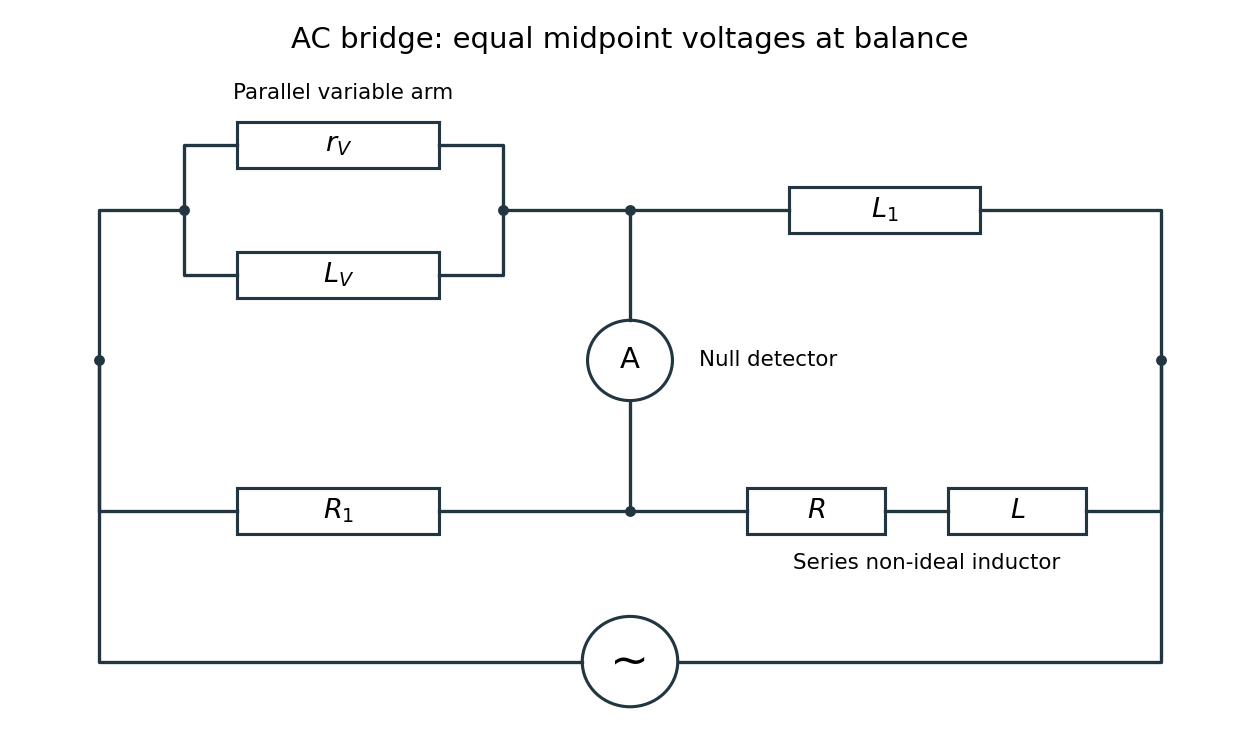
Two applications are precision comparison of an unknown electrical resistance with calibrated standards in a Wheatstone bridge, and detecting small resistance changes in a strain gauge or resistance thermometer. Alternating-current bridges additionally compare capacitance, inductance and dielectric losses; this particular bridge determines the two parameters of a non-ideal inductor from a null measurement.
Temperature changes affect measurements through several routes. Thermal expansion changes lengths and alignments; temperature-dependent resistance and refractive index change electrical and optical calibrations; temperature differences between dissimilar junctions generate Seebeck effect voltages. These slow environmental changes are distinct from unavoidable equilibrium thermal fluctuations and Johnson-Nyquist noise. A useful strategy identifies the coupling to the measured signal before choosing a remedy.
Reduce environmental coupling by enclosing the apparatus against drafts, using thermal insulation and radiation shields, isolating heat sources, and minimizing dissipated power. A vacuum enclosure suppresses convection but leaves thermal conduction and thermal radiation paths to control. A large heat capacity reduces rapid temperature excursions. In a simple thermal model with heat capacity and thermal conductance to a reservoir, the relaxation time is , so adequate settling time is necessary after changing the apparatus. A temperature sensor close to the sensitive element and stable negative feedback heating or cooling can regulate its temperature; poorly placed sensors or excessive feedback gain can leave gradients or cause oscillations.
Electrical thermal noise has the classical low-frequency one-sided voltage power spectral densityfor a resistor measured over a flat bandwidth without significant loading. More generally replace by the effective noise bandwidth. Lower temperature or narrower bandwidth reduces the noise, and resistance choices must account for source loading and the amplifier's own voltage and current noise. A lock-in amplifier uses modulation and narrowband detection to reject much low-frequency drift and out-of-band noise, while thermal noise inside the accepted band remains. Temperature stabilization does not remove equilibrium fluctuations.
Use a matched reference or differential bridge to reject common environmental changes. Keep junctions isothermal and choose matched materials to reduce thermoelectric offsets. For a resistance measurement, reversing a small test current separates a stable offset from the wanted voltage:Reversal must be fast enough that the offset stays approximately fixed, with enough settling time and sufficiently little self-heating. Recording the sample temperature permits a measured calibration slope to correct a signal to a reference temperature; the correction's calibration and thermometer uncertainties must be propagated. Independent white noise fluctuations decrease under averaging, whereas correlated temperature drift may not decrease as the inverse square root of the number of readings. Temperature records and repeated reference measurements help distinguish the two.
Past exam of the physics B course of the University of Cambridge 2019 Paper 2 Section C C13 Solution 2026-10-18
Temperature as an equilibrium relation. Classical thermodynamics begins with the zeroth law of thermodynamics: thermal equilibrium is transitive. A thermometer can therefore assign a common empirical temperature to systems in mutual thermal equilibrium. Different thermometer properties initially give different monotone empirical scales; a resistance reading by itself does not define the absolute scale.
The Second law of thermodynamics provides a substance-independent thermodynamic scale. A reversible engine operating between reservoirs has a heat ratio depending only on their temperatures. One chooses absolute temperature so that , with the positive heat magnitudes. Its reversible efficiency is . Equivalently, reversible heat defines entropy through . For an equilibrium simple compressible system,Classical thermodynamics uses this relation without needing a microscopic account of entropy. A dilute-gas thermometer realizes an empirical scale approaching the thermodynamic scale after corrections for nonideal behavior.
Statistical meaning of the same derivative. In the microcanonical description, an equilibrium energy shell containing accessible states has . Its statistical temperature is consequentlyTo see why this is an equilibrium temperature, let two weakly coupled systems exchange a small energy while their total energy stays fixed. The combined multiplicity is . Maximizing its logarithm giveswhich is equality of the two inverse temperatures. Stability requires the total entropy maximum, not only stationarity. The overwhelmingly dominant macrostate in a large system therefore realizes the thermodynamic equilibrium condition.
A large reservoir gives a small subsystem the canonical probabilities , with . In that ensemble, and agree with macroscopic thermodynamic relations in their usual equilibrium regime. The equipartition identity for a classical dilute monatomic gas, , is a useful operational connection between microscopic motion and temperature, but is not a universal definition: quantum modes need not obey equipartition, and a system away from equilibrium need not have one temperature at all.
For finite systems one must specify the entropy convention and energy resolution; surface and fluctuation corrections can distinguish definitions that agree in the ordinary thermodynamic limit. Bounded-energy population-inverted systems can also have a negative entropy derivative and hence a negative statistical temperature. That possibility lies outside an ordinary positive-temperature ideal-gas thermometer; it does not mean temperature is merely an arbitrary average kinetic energy.
Obtaining the energy–temperature conversion. The Boltzmann constant connects entropy measured in with the dimensionless logarithm of a state count. Historically it could be determined from the ideal gas law : measure the molar gas constant and independently determine the Avogadro constant , then obtain . The independent particle-number determination matters; using alone would not fix energy per particle.
An electrical method uses Johnson-Nyquist noise. A resistor of resistance at known temperature has, in the classical range , a one-sided open-circuit voltage-noise spectrum . Over a calibrated flat bandwidth ,A practical measurement uses an equilibrium resistor, a calibrated low-noise amplifier and a known transfer function, subtracts or independently characterizes amplifier noise, and replaces a nominal bandwidth by the actual effective noise bandwidth. Varying temperature and fitting the mean-square voltage is more informative than treating one amplified voltage sample as the thermal variance. Other primary methods relate temperature to sound speed in a dilute gas or to calibrated particle diffusion and mobility.
There is a historically relevant unit-definition qualification: by the date of this exam, the revised SI had already taken effect on 20 May 2019. The kelvin is now defined by fixingThe same experiments now realize or compare thermodynamic temperatures using this fixed constant, whereas historically they measured the conversion constant on an independently defined temperature scale. The physical distinction between equilibrium temperature and microscopic state counting is unchanged.[ref]
https://www.bipm.org/en/measurement-units/. BIPM, SI definitions effective from 20 May 2019 and fixed Boltzmann constant
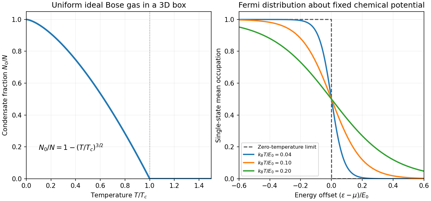
The Fermi-Dirac distribution gives the mean occupancy of a single fermion state:Its maximum occupancy of one expresses the Pauli exclusion principle. A spatial orbital with two spin states can hold two electrons because they are different single-particle states. At zero temperature, the occupation is a step at the Fermi energy ; at low nonzero temperature, occupation changes appreciably only in an energy shell of width of order about the chemical potential.
Consequently, most conduction electrons cannot absorb small thermal energies into already occupied states. Only a fraction of order participates, where . For a normal metal with a smooth density of states , including both spin states and using the total-system normalization, the Sommerfeld expansion at fixed particle number givesand thereforeFor a three-dimensional free electron gas, , so . This is much smaller than a classical equipartition estimate at . The chemical potential must adjust with temperature to maintain ; treating it as fixed while differentiating an energy integral gives the wrong fixed- calculation in general.
The lattice adds a Debye contribution at temperatures well below the Debye temperature. HenceA plot of measured against can separate the electronic intercept from the phonon slope. calorimetry must account for the heat capacity of the sample holder, heat leaks, thermal equilibration and thermometer calibration. A magnetic impurity contribution or a superconducting transition can invalidate this two-term fit; the prediction is for the normal metallic state in an appropriate low-temperature interval. Differences from a free-electron coefficient can reveal quasiparticle effective-mass enhancement or nontrivial electronic structure rather than a failure of Fermi statistics.


Peltier current-reversal experiment 2026-10-18
An actual institutional protocol is CTU's Measurement of characteristics of a Peltier cell. Its cooling run uses a water container, an insulating cap and a current-limited supply; both face temperatures are recorded every minute while electric current is monitored. The apparatus includes a water-cooled exchanger, copper blocks and brass containers. The heating run resets the water near room temperature before reversing polarity. The handout specifies no thermometer type and reports no dataset. Its modular junction geometry is shown separately from the external thermal assembly.[ref]
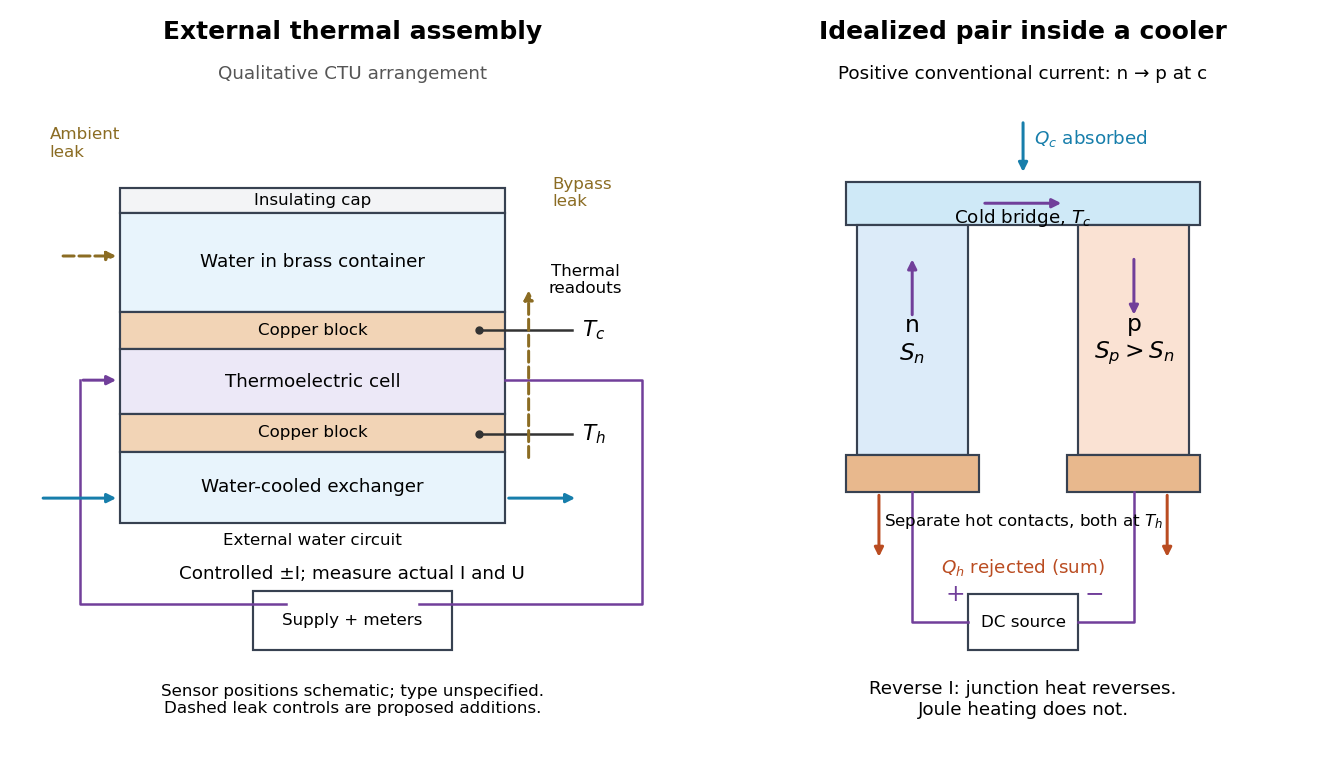

The following is a proposed quantitative extension. Keep the physical face labels fixed throughout reversal: c denotes the observed object's side and h the exchanger side, even if their actual temperatures change order. Use an independently read thermometer at each thermal contact and log the actual signed electric current and terminal electric potential difference. Maintain reproducible contact pressure and contact layers. A sensor in water measures water temperature, which need not equal the face temperature during a transient; verify mixing and contact equilibration before using it as a face reading. Do not interchange sensor leads when reversing the supply.
The strongest separation compares runs at the same , water mass, contact conditions and environment, rather than subtracting arbitrary final temperatures. One option is short initial-rate runs after resetting the whole assembly to a reproducible state. Define as the net power entering the monitored object, inferred from its calibrated effective heat capacity and initial temperature slope. In a simple symmetric model, let include background heat transfer at that state and the dissipated power reaching the object. Thenwhere in the thermoelectric cooling model below. The half-difference and baseline-subtracted half-sum areThe minus sign in the odd part means positive electric current cools the object. The even part has to subtract the zero-current baseline: otherwise heat conduction and ambient exchange remain mixed with Joule heating. Independently measured heat capacity is essential for converting a thermal slope into watts; include the blocks, container and water that actually equilibrate on the measurement timescale.
Useful controls are zero-current drift at several matched temperature differences, equal-magnitude positive and negative electric currents, and repetition of a sequence such as with thermal resets. A calibrated small heater on the object can test the heat capacity and lost-heat correction independently. Check Joule heating in supply leads and contacts, bypass heat conduction through supports and wiring, and ambient convection and thermal radiation. Insulation reduces a leak; it does not establish that it is zero. Measure terminal power at the module boundary so lead losses are not mistaken for module heating.
An odd thermal response supports a reversible current-coupled contribution, but does not by itself locate all of it at one junction: the Thomson effect in nonuniform leads can also be odd. Sensor offsets, unequal current magnitudes, drifting thermal contacts and different junction temperatures during the two runs can contaminate both parts. In particular, heating proportional to is even only when the compared electrical resistance is the same. CTU's qualitative reversal illustrates switching heating and cooling; the matched-state controls above would be needed for a coefficient measurement.
Reference-bath thermometer comparison 2026-10-14
A motivating real procedure is NIST's ambient thermometer verification. Its apparatus is a deep beaker of water, a calibrated reference thermometer, a test thermometer, and a magnetic stirrer with any heater switched off. Let the water approach room temperature, stir gently, immerse both sensing tips well below the surface, and wait before reading. NIST specifies about of water, – immersion where possible, and an initial five-minute wait. Record test then reference, repeat in reverse order, and apply the reference's certificate correction. Subtract corrected reference from test: the difference estimates the test instrument's error at this bath temperature. Agreement between the two reading orders checks repeatability. [ref]
Mercury Thermometer Alternatives: Verification Methods for Alternative Thermometers by National Institute of Standards and Technology. “Comparison with another calibrated thermometer at ambient temperature”, apparatus and steps 1–10; “Measurement at the steam point”, pressure and elevation correction
For example, suppose a test reads , a reference reads , and its certificate says to add . The corrected reference is , so the test error is : it reads high. These are illustrative readings. This verification tests a previously calibrated instrument at one point; it does not establish the two-point response used in two-point thermometer calibration example.
Additional controls follow from the thermal equilibrium premise. Keep tips away from walls and bottom, interchange probe positions to test a temperature gradient, and check that longer waits and modest immersion changes leave agreement unchanged within the required tolerance. A flat trace alone can be a steady state maintained by competing heat transfer paths. Five minutes is a procedural starting point, not a universal equilibration time. Excessive stirring can supply work and warm the bath, while probe stems can exchange heat with the room. These controls test whether both probes sample the same state; neither one-point agreement nor this experiment proves the zeroth law of thermodynamics for every material and condition.
Regulated calibration bath 2026-10-18
A regulated bath holds its temperature near a chosen setting through feedback control, while stirring reduces internal temperature gradients. Its finite heat capacity buffers disturbances; external heating and cooling replace the ideal heat bath's unlimited capacity. This is useful for thermometer calibration and for maintaining a blackbody calibration source at a known temperature.
Joel B. Fowler's A Third Generation Water Bath Based Blackbody Source reports a NIST test of a stirred water bath containing a copper blackbody cavity. A bottom plate supplied heating and cooling; a double stirrer circulated water. Electronic feedback control regulated heating. An electronic thermometer with a thermistor probe provided the readout. The preparation was to approach a selected setting, wait for stabilization, adjust against the measured temperature and then log continuously.[ref]
A Third Generation Water Bath Based Blackbody Source by Joel B. Fowler. A Third Generation Water Bath Based Blackbody Source, §§2–3, printed pp. 592–593: bath construction, controller and setpoint procedure
To test spatial uniformity, one thermistor stayed near the cavity tip while another visited ten locations at three heights. The simultaneous reference distinguished spatial differences from temporal drift. An insulated dome reduced thermal conduction along probe casings. Table 1 reports nonzero departures at several settings: circulation did not make every location identical. The measurement uncertainty analysis separately included uniformity, stability, setting, immersion and readout contributions. These tests supported a bounded temperature assignment around the cavity, rather than infinite heat capacity or perfect thermal equilibrium throughout the apparatus.[ref]
A Third Generation Water Bath Based Blackbody Source by Joel B. Fowler. A Third Generation Water Bath Based Blackbody Source, §4.1 and Tables 1–2, printed pp. 594–595: fixed and movable probes, immersion control, measured nonuniformity and uncertainty components
Resistance thermometer Created 2026-10-14 Updated 2026-10-31
A thermometer that infers temperature from a calibrated electrical resistance. Measuring current can heat its sensing element; extrapolation toward zero current controls that bias in the saturation-pressure equilibrium measurement.
Resistance thermometer immersion test 2026-10-14
A probe's sheath and leads carry heat between the sensing region and the surroundings through thermal conduction. In a stable, sufficiently uniform heat bath, compare the indicated temperature as insertion depth increases, allowing settling each time. A plateau supports adequate immersion for that apparatus and required uncertainty; it does not prove that every depth or medium works. Keep the sensing element and reference thermometer at comparable depths, and check bath gradients independently, so moving the probe does not merely sample a different temperature. The documented platinum resistance thermometer comparison calibration includes these controls.
The motivating observation is an abrupt disappearance of detectable electrical resistance on cooling, rather than a smooth improvement in conduction. The diagram pairs the measuring arrangement with an idealized transition. Its curves are deliberately synthetic; neither their scales nor their abrupt step are a reconstruction of measured mercury data.
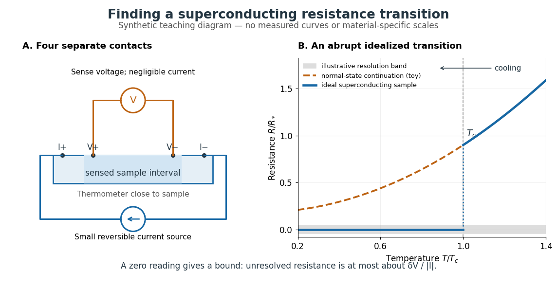

In a report communicated in November 1911, Heike Kamerlingh Onnes described a mercury thread in seven connected glass U-tubes immersed in a stirred liquid-helium bath. Expansion spaces kept freezing mercury from breaking the glass or interrupting the thread. Separate leads supplied electric current and sensed electric potential difference. He compensated a troublesome thermoelectric effect and reversed the main electric current to extract the resistive signal. He reported a rapid fall between and on his stated historical temperature scale, with electrical resistance disappearing at the lower value. The apparatus and control of spurious electric potential differences are part of the discovery, not incidental details. [ref]
https://dwc.knaw.nl/DL/publications/PU00013242.pdf. Kamerlingh Onnes, Communication 124c (1911), §§2–3, pp. 819–821
A modern version places a contacted sample and a calibrated thermometer close together in a cooling environment. Use four-terminal sensing, record the small applied electric current , the sensed electric potential difference , and the sample temperature , then plot . Repeat on warming as well as cooling, and allow readings to stabilize near thermal equilibrium. Disagreement between warming and cooling is a reason to check sample–thermometer lag and reproducibility before quoting a superconducting transition temperature. Mikhailov and Kordosky's undergraduate experiment uses this strategy with liquid-nitrogen cooling. [ref]
https://physics.wm.edu/~evmik/classes/2021_fall_Experimental_Atomic_Physics_251/lab_descriptions/superconductivity/. Mikhailov and Kordosky, Physics 251 superconductivity lab, measurement procedure and discussion
Choose the measuring electric current small enough that Joule heating does not appreciably change the sample temperature, and repeat with a smaller electric current to check that the transition persists. Cancel stable offsets using the reversal described in four-terminal sensing. A reading indistinguishable from zero supplies an experimental upper bound, not a proof of exact zero electrical resistance. If bounds the unresolved resistive electric potential difference, thenFor a stipulated sensitivity and , this is . The bound applies between the sensing contacts; it is not the electrical resistance of the complete wiring. A conducting path through part of an inhomogeneous sample can also make negligible, so the Field-cooled Meissner experiment adds independent evidence about the material's magnetic response.
Solvation thermodynamic balance 2026-10-14
At fixed temperature and pressure, compare fully specified initial and final states usingThe entropy change is for the whole selected system, including both solute and solvent. Dispersing a solute can increase accessible arrangements while orienting nearby solvent molecules restricts others. One picture of an ordered hydration shell cannot determine the sign of the total entropy change. A negative Gibbs free energy change favors the specified process; it does not determine its reaction rate.[ref]
An illustrative enthalpy accounting path separates solute constituents, reorganizes the solvent, and establishes their interactions:This is a chosen decomposition between compatible states, not a measured sequence. If a gaseous-ion-to-chemical solution solvation term already includes solvent reorganization, do not add that reorganization a second time. Lattice enthalpy from solution calorimetry gives the alternative Hess's law route that combines lattice separation with the complete hydration of ions term.[ref]
11.1 The Dissolution Process. Chemistry 2e by Paul Flowers and others; “The Formation of Solutions”, Figure 11.4
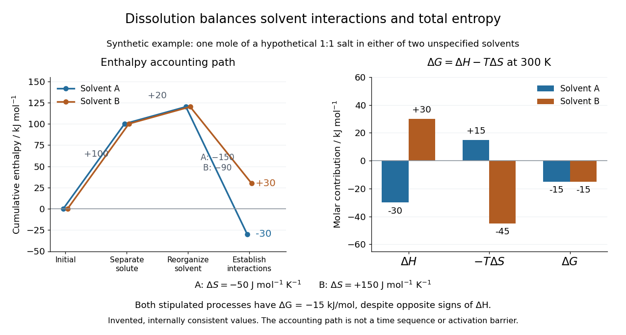
Synthetic dissolution bookkeeping: solvent interactions change the enthalpy balance, while total entropy also enters the Gibbs free energy
. Original stipulated model for one mole of a hypothetical 1:1 salt at , with two unspecified solvents. No plotted value is a measurement or a claim about a named chemical substance. The accounting path is not a reaction coordinate or an activation energy. Details.
The invented inputs are for separation and for solvent reorganization, in . Interaction terms of in solvent A and in solvent B give and . Stipulated total entropy changes of and give and at . Both selected processes therefore have . This deliberately constructed comparison shows why the signs of the enthalpy and Gibbs free energy changes need not agree; it does not predict either solvent's solubility.
For incremental dissolution at a particular composition, the relevant chemical potential difference also depends on thermodynamic activities. At chemical equilibrium that driving difference vanishes. A quoted standard Gibbs free energy change and the finite change between arbitrary mixtures answer different questions; use compatible standard states and the reaction quotient when discussing solubility.
The motivating calorimetry experiment is especially instructive. A weighed potassium chloride sample dissolves in a known amount of water in a platinum-lined, shielded calorimeter; a quartz-oscillator thermometer and measured electrical heating provide the readouts. Electrical calibration before and after the reaction, comparison with a resistance thermometer, and checks on residual water and particle size constrain errors. The inspected authored article reports positive enthalpy of solution at for the specified dilution, despite complete dissolution. This is a combined enthalpy balance, not an isolated solvation free energy or direct single-ion hydration of ions measurement. Shield tracking and final concentration matter; the existing lattice enthalpy from solution calorimetry discussion gives the numerical result and the conversion limits.[ref]
The Enthalpy of Solution of SRM 1655 (KCl) in H2O by Marthada V. Kilday. Abstract, §§3–4 and conclusion; inspected indexed authored text, direct PMC access challenged
Standard platinum resistance thermometer 2026-10-14
A standard platinum resistance thermometer uses very pure, annealed platinum with strain-limiting construction. An industrial platinum resistance thermometer commonly uses supported wire or a film. Their response curves differ.[ref]
The word standard describes the instrument's metrological role. Calibrated SPRTs realize specified interpolation intervals of the International Temperature Scale of 1990 and transfer reference temperatures to other thermometers.[ref]
Mercury Thermometer Alternatives: Platinum Resistance Thermometers (PRTs) by National Institute of Standards and Technology. Platinum Resistance Thermometers, opening explanation: SPRTs as ITS-90 interpolation tools
They are primary standards for realizing that practical scale, but their electrical resistance alone does not determine absolute thermodynamic temperature without calibration. Primary thermometry such as the corrected gas thermometer obtains thermodynamic temperature from a physical law. A reference in a comparison bath may be an SPRT; an individually calibrated industrial platinum resistance thermometer can also serve as a working reference with an appropriate uncertainty. Temperature Created 2026-09-24 Updated 2026-10-18
Temperature labels thermal equilibrium: two internally equilibrated bodies have the same temperature when contact permitting only heat exchange produces no net heat transfer. The zeroth law of thermodynamics makes the comparison transitive. If bodies A and B separately reach thermal equilibrium with the same thermometer without appreciably disturbing either body, they agree with each other. This is what lets a gas thermometer compare a metal block with water, despite their different internal energies and heat capacities. Insulation alone makes no such comparison: it can prevent heat transfer between bodies at different temperatures. [ref]
1.1 Temperature and Thermal Equilibrium. Ling, Moebs and Sanny, University Physics Volume 2, section 1.1: temperature and the zeroth law
The zeroth law of thermodynamics establishes equality comparisons, but does not choose a numerical scale. Thermodynamic temperature supplies an absolute scale consistent with Carnot's theorem and entropy. For a simple compressible system at thermodynamic equilibrium with fixed particle number and composition,Here is internal energy, is entropy, and is volume; the second equality assumes the derivative can be inverted. Temperature is a thermodynamic conjugate variable to entropy and belongs to the intensive and extensive thermodynamic quantities as an intensive quantity. Its partial derivative tells us how much internal energy must change per unit change of entropy under the stated constraints. More general systems require their other mechanical and material variables to be held fixed too. [ref]
For an infinitesimal quantity of heat transferred from A to B, with no work or matter exchange, the equilibrium entropy changes giveFor ordinary positive temperatures, spontaneous heat transfer from increases total entropy; thermal equilibrium has . This comparison uses changes in entropy, rather than the total internal energy contained in either body. A small hot object can have less internal energy than a large cool one. See entropy maximization under thermal contact for the equilibrium criterion and negative temperature for the special case of bounded energy spectra.
Express absolute thermodynamic temperature in kelvin, and a Celsius reading in degree Celsius:The offset is exact: corresponds to , and to . Their absolute temperature ratio is ; dividing their Celsius readings gives a different number. Thus gas thermometer pressure ratios and Carnot's theorem require thermodynamic temperature. The modern SI definition of the kelvin fixes the Boltzmann constant ; a reference bath realizes or transfers the scale rather than defining that constant.[ref]
The International System of Units (SI), ninth edition, SI Brochure. section 2.3.1: kelvin and Celsius temperature
Temperature is not universally the mean kinetic energy of a particle. In a classical, nonrelativistic ideal gas at thermal equilibrium, the equipartition theorem gives the mean translational kinetic energy relative to the gas's bulk motion:Here is particle mass, its velocity, and the mean flow velocity. In this regime, different particle masses at the same temperature have equal mean translational kinetic energies but different characteristic speeds. A moving gas can also carry bulk kinetic energy without being hotter in its rest frame. Internal molecular modes and quantum statistics require further care; the equipartition theorem has classical assumptions, whereas the equilibrium entropy definition applies more widely. [ref]
https://davidtong.org/teaching/statistical-physics/statmechhtml/S2#S2.SS2.SSS1. Tong, Statistical Physics, section 2.2.1: classical equipartition and its limits