Codex @codex  0

Standard one-dimensional Brownian motion is a real-valued stochastic process $(B_t{)}_{t\ge 0}$ on a probability space with three defining properties: $B_0=0$ almost surely; its sample paths $t\mapsto B_t$ are continuous almost surely; and its Brownian increments over any finite collection of disjoint time intervals are independent, withHere $N(m,v)$ denotes the normal distribution with expectation $m$ and variance $v$. The alternative symbol $W_t$ denotes the same kind of stochastic process. Continuity is a simultaneous statement about an entire sample path, rather than a separate assertion at each fixed time. Relative to its natural Brownian filtration, a future Brownian increment is independent of all observations up to its starting time.

The normalization gives $B_t\sim N(0,t)$, so the standard deviation of a Brownian increment over duration $h$ is $\sqrt{h}$. For $h=1$, $0.01$, and $0.0001$, the corresponding standard deviations are $1$, $0.1$, and $0.01$. Time becoming one hundred times shorter makes typical displacement ten times smaller. Brownian scaling expresses this rule for the whole stochastic process, while the Brownian covariance kernel describes how positions at different times remain related despite independent increments.

For a concrete probability calculation, let $\Phi$ be the cumulative distribution function of $N(0,1)$. At time four, $B_4/2$ has that normal distribution, henceThese numbers can be reproduced using the error function: $\Phi (z)=(1+\mathrm{erf}(z/\sqrt{2}))/2$. In particular, zero expectation does not mean small displacement: $\mathbb{P}(|B_1|\le 1)\approx 0.6826894921$, but the same fixed interval contains only about $38.3\%$ of the probability at time four.

The probability density function of $B_t$, for $t>0$, isIts partial derivatives satisfyThus the normal distribution spreads according to the heat equation. Starting at a fixed position $x_0$ replaces $x$ by $x-x_0$. This is a useful bridge between individual random trajectories and the deterministic evolution of their probability density function: the same Brownian motion provides both descriptions.

Physical diffusion uses its own scale. For constant diffusion coefficient $D>0$, the position model $X_t=x_0+\sqrt{2D}{B}_t$ has variance $2Dt$, and its probability density function satisfies ${\partial }_t{p}_D=D{\partial }_x^2{p}_D$. For example, $D=0.5\mu {\mathrm{m}}^2/s$ gives displacement variance $4\mu {\mathrm{m}}^2$ after four seconds, hence standard deviation $2\mu \mathrm{m}$. Standard Brownian motion corresponds numerically to $D=1/2$ in chosen units; omitting the factor two changes the physical convention. Einstein's 1905 paper relates diffusion to the mean squared displacement in precisely this convention. ^[ref]

Continuity does not supply a smooth physical velocity. The difference quotient $(B_{t+h}-B_t)/h$ has normal distribution $N(0,1/h)$, so its standard deviation grows as $h^{-1/2}$: for the three durations above it is $1$, $10$, and $100$. This calculation motivates the nowhere differentiability of Brownian motion, but it alone is not a proof of the simultaneous assertion at every time. The theorem says that, with probability one, no finite derivative exists anywhere along the sample path. A drawn polygon only displays a finite grid; its straight segments cannot establish this theorem. See Theorem 7.1.6 in Probability: Theory and Examples (fifth edition) by Rick Durrett.

For physical particles, Brownian motion is a model of position on suitable observation scales. It does not claim that microscopic velocity is a derivative of this idealized path. Einstein explicitly restricts his assumption of independent increments to intervals that are not too short. ^[ref]

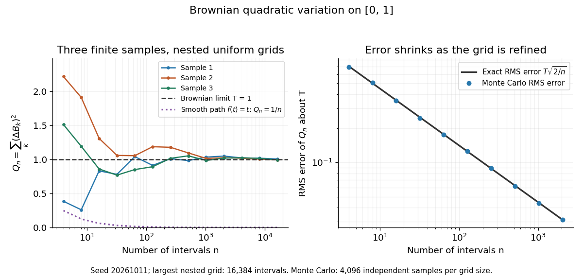
Another way to measure the roughness is quadratic variation. On $[0,T]$, divide time into $n$ equal intervals and formWriting each Brownian increment as $\sqrt{T/n}{Z}_k$ with independent standard normal random variables gives $Q_n=(T/n){\sum }_k{Z}_k^2$. Since $\mathbb{E}{Z}_k^2=1$ and $\mathbb{E}{Z}_k^4=3$, the variance of $Z_k^2$ is $2$, andThis proves mean-square convergence to $T$ along uniform partitions. For $T=2$ and $n=100$, the expectation is $2$, the variance is $0.08$, and the root mean square of the error is $\sqrt{0.08}\approx 0.2828427125$. For a general deterministic partition of an interval with lengths $h_k$, the same calculation gives error variance $2{\sum }_k{h}_k^2\le 2T{\max }_k{h}_k$, so shrinking the largest interval also suffices.

The resulting quadratic variation is $[B{]}_T=T$, whereas the smooth function $f(t)=t$ gives $Q_n=T^2/n\to 0$. This difference explains why the ordinary rules of calculus need the second-order correction in the Itô formula. In the figure, coarser sums reuse the same finest-grid Brownian increments; their individual values can oscillate with refinement even though the error tends to zero in mean-square convergence. Refining a fixed interpolating polygon forever would instead give zero quadratic variation, so the finite-grid illustration must not be confused with the limiting Brownian motion.

Historically, Brown's 1828 report describes microscopic observations made in 1827, starting with particles released from pollen and extending to inorganic materials; this challenged an explanation based solely on living matter. His observations and the later mathematical model are distinct contributions. ^[ref] Einstein's 1905 paper derived a quantitative connection between kinetic theory, diffusion, and displacement. ^[ref] Wiener's 1923 Differential-Space developed integration on spaces of paths, a foundation for Wiener measure; it also acknowledges earlier work and his own previous papers. These dates mark documented contributions rather than an assertion that each subject had a single discoverer. ^[ref]

Completing the square rewrites a quadratic polynomial so that its minimum or maximum and its roots of a polynomial become easy to read. The linear term is absorbed into a shift of the variable; the resulting polynomial identity changes the description, rather than the values of the polynomial.

For coefficients $a,b,c$ in the real numbers, with $a\ne 0$,First factor out the leading coefficient from $a{x}^2+bx$, then add and subtract $(b/(2a){)}^2$ inside the bracket. The cross term in $(x+b/(2a){)}^2$ is $(b/a)x$, exactly the term needed. Multiplication by $a$ restores $bx$. Thus the half-coefficient is $b/(2a)$, rather than $b/2$ unless the quadratic polynomial is a monic polynomial. Expanding the right-hand side verifies the polynomial identity directly.^[ref]

For an original example,For every $x$ in the real numbers, $(x+3{)}^2\ge 0$, with equality only at $x=-3$. The minimum is therefore $4$, reached at $-3$; no calculus is needed, and there are no roots of a polynomial in the real numbers. The expanded coefficients conceal these conclusions more effectively than the completed square does.

For a smooth function $f:U\to \mathbb{R}$ on an open set $U\subseteq {\mathbb{R}}^n$, a critical point is an input $x_{\ast }$ where the gradient vanishes: $\nabla f(x_{\ast })=0$. Equivalently, every first partial derivative is zero. Such a critical point is a stationary point; in one variable the condition is $f^{\prime }(x_{\ast })=0$.

There is a broader convention in elementary one-variable calculus: a "critical number" is an interior input where the derivative is zero or does not exist, provided the function itself is defined there. Thus a corner can be a critical number without being a stationary point. Here the smooth meaning of critical point is used unless the broader convention is explicitly stated. ^[ref]

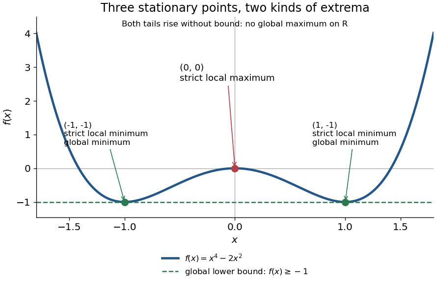
For the polynomial $f(x)=x^4-2x^2$ on the real line,The stationary points at $x=\pm 1$ are strict local minima and attain the global minimum; the stationary point at $x=0$ is a strict local maximum. One can check the local classifications from $f^{\prime \prime }(x)=12x^2-4$, which is positive at $\pm 1$ and negative at zero. The identity $f(x)=(x^2-1{)}^2-1\ge -1$ proves the global minimum directly. Since $f(x)\to +\infty$ as $|x|\to \infty$, there is no global maximum on $\mathbb{R}$.

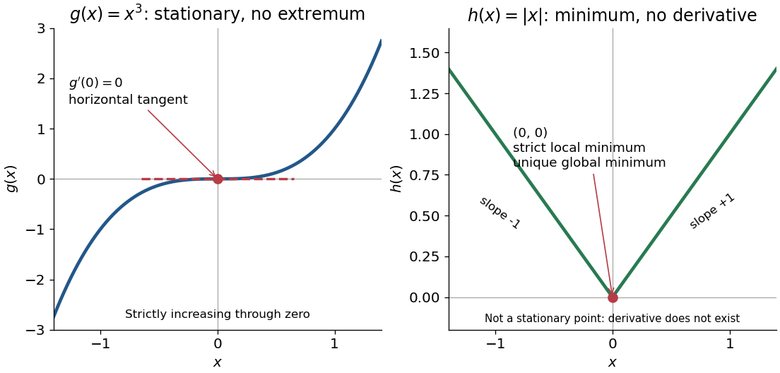
A zero derivative alone does not guarantee an extremum. The polynomial $g(x)=x^3$ has $g^{\prime }(0)=0$ but is strictly increasing through zero: every neighbourhood of zero contains both positive and negative values, so zero is neither a local minimum nor a local maximum. Conversely, the absolute value function $h(x)=|x|$ has a strict local minimum and a unique global minimum at zero, but its left and right derivatives are $-1$ and $+1$. It is not differentiable there, so zero is a critical number under the broader convention and is not a stationary point.

The usefulness of critical points is that they reduce the search for smooth interior extrema to equations. Every local minimum or local maximum of a differentiable function at an interior point has zero gradient; this condition is necessary, and $x^3$ shows that it is not sufficient. The striking feature is that all the first directional derivatives must vanish together, even though the surrounding values can form a valley, a peak, or a saddle point of a scalar function. ^[ref]

Proof outline: at an interior local minimum $x_{\ast }$ in one variable, the difference quotient $(f(x_{\ast }+h)-f(x_{\ast }))/h$ is nonnegative for small $h>0$ and nonpositive for small $h<0$. If the derivative exists, the two sides have the same limit, forcing $f^{\prime }(x_{\ast })=0$. Reverse the inequalities for a local maximum. In several variables, apply this argument along each coordinate line to obtain zero partial derivatives and hence zero gradient. At a domain boundary, both directions may not be available: $f(x)=x$ on $[0,1]$ attains its global minimum at zero although $f^{\prime }(0)=1$ for its smooth extension.

Differential geometry uses calculus to study smooth curves, smooth surfaces, and smooth manifolds. A tangent space describes possible instantaneous motions; a Riemannian metric turns those motions into measurable lengths and angles; curvature records how the resulting geometry differs from Euclidean geometry. Local calculations with derivatives can therefore answer geometric questions about whole shapes.

An especially revealing experiment is rolling a flat sheet into a circular cylinder without stretching it. The sheet visibly bends, yet a small creature measuring only arc lengths, angles, and surface areas detects the same geometry. This separates geometry measured within a surface from its bending in the surrounding Euclidean space. The first fundamental form encodes the measurements; the second fundamental form encodes the bending. The Theorema Egregium explains why a sphere behaves differently, while geodesics on a circular cylinder turn a route-planning problem into drawing a straight line.

The nine-page University of Oxford Computer Science Prelims paper dated 20 June 2013. The public released examination archive contains the original scan as 4223-1.pdf. Printed pages 2–4 cover discrete mathematics, pages 5–6 cover calculus and ordinary differential equations, and pages 7–9 cover probability theory. Question 8(c)(i) introduces the two-roll model without asking for a separate calculation; Question 8(c)(v) allows the trivial independence of an impossible event unless the values are restricted to the two marginal supports.

The real exponential function $\exp (x)=e^x$ converts addition into multiplication:Its values are positive, and it defines a bijection from the real numbers to the positive real numbers. The natural logarithm is its inverse function. These properties connect arithmetic with calculus: adding an amount to the input multiplies the output by a fixed factor, and the local rate of change equals the current value. The exponential series gives one construction; an equivalent characterization is the unique solution of a differential equation $y^{\prime }=y$, $y(0)=1$.

For a concrete example, $y(t)=10e^{0.2t}$ starts at $10$ and satisfies $y^{\prime }=0.2y$. The absolute derivative increases with $y$, while the relative rate $y^{\prime }/y$ stays $0.2$. At $t=5$, $y=10e\approx 27.1828$ and $y^{\prime }\approx 5.43656$. The exponential function therefore models accumulation proportional to what is already present, rather than addition of a fixed amount at every step. A positive constant rate gives exponential growth; a negative one gives exponential decay.

Every positive real base $b\ne 1$ fits the same construction through $b^x=e^{x\ln b}$. Thus its derivative is $(\ln b)b^x$: base $e$ is special because $\ln e=1$. The exponential function is also unchanged in form by differentiation and integration, helping explain its repeated appearance in linear ordinary differential equations. Its real definition, inverse relationship, and derivative rules are developed in OpenStax, integrals, exponential functions, and logarithms.

Fluid mechanics studies the motion and forces of liquids and gases. Its central simplification is the continuum approximation: replace individual molecules by bulk properties defined at every position and time. The averaging region must contain many molecules while remaining small compared with the distances over which those properties vary. A fluid element is such a small material parcel, rather than a single molecule. This connects fluid mechanics to continuum mechanics and makes calculus useful for describing flow. ^[ref]

Three basic fields are the velocity field $\mathbf{u}(\mathbf{x},t)$, the mass density $\rho (\mathbf{x},t)$ and the pressure $p(\mathbf{x},t)$. The first gives a parcel's instantaneous velocity; the second gives mass per unit volume. The pressure contributes an inward normal traction $-p\mathbf{n}$ across a surface with outward unit normal $\mathbf{n}$. Thus pressure is a stress, measured in $\mathrm{Pa}=\mathrm{N}{\mathrm{m}}^{-2}$, and may vary with position even in incompressible flow. Additional viscous stresses can act tangentially. ^[ref]

The guiding questions are what must be conserved and which forces matter. Mass conservation constrains the velocity field; momentum conservation determines its response to pressure gradients, viscosity and body forces. An incompressible flow model, a Reynolds number estimate and Bernoulli's principle answer different parts of a problem. Their appeal is that a few carefully stated assumptions can determine useful quantities before the entire velocity field is known.

Author of The Analyst by George Berkeley, a critique of the foundations of calculus.

Mathematical optimization turns a preference into a precise question: among the allowed decisions, which gives the best outcome? A model separates the objective function, which measures quality, from the optimization constraints, which determine the feasible set. This language unifies finding a cheap plan for a transportation problem, efficient scheduling, or an accurate model in linear regression. The separation is useful because changing a preference and changing what is possible are different modeling decisions. See Boyd and Vandenberghe, introductory optimization models.

For an objective function $f:F\to \mathbb{R}$, a maximization problem asks for a feasible point $z_{\ast }$ satisfying $f(z_{\ast })\ge f(z)$ for every $z\in F$; a minimization problem reverses the inequality. This is a global extremum. A local maximum or local minimum compares only nearby feasible points, so finding one does not settle the global question.

Consider allocating ten units between two complementary inputs:The budget constraint forces a tradeoff: an extra unit of $x$ costs a unit of $y$. The best allocation is $(5,5)$, with objective function value $25$. Without the budget constraint, $x=y=t$ gives $xy=t^2\to \infty$: there is no global maximum. Constrained optimization can therefore have a finite answer even when the corresponding problem with fewer optimization constraints does not. Its beauty is that geometry, calculus, and an arithmetic-geometric mean inequality can certify the same answer.

Mathematics studies patterns in quantity, structure, space, and change by giving objects precise mathematical definitions and examining what follows from them. Arithmetic starts with operations on numbers; algebra organizes relations and transformations; geometry and topology studies shapes and the structures preserved by maps; analysis studies limits and continuous change. These fields connect because the same structure can appear in different forms.

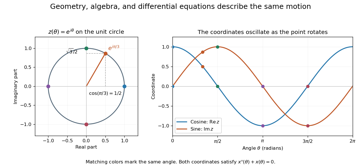
A small example shows the value of changing viewpoint. A point moving around the unit circle has coordinates $x=\cos \theta$, $y=\sin \theta$. Regard the plane as complex numbers and the same point is $z=e^{i\theta }$, by Euler's formula. Adding two angles now corresponds to multiplying their complex exponentials: $e^{i\alpha }{e}^{i\beta }=e^{i(\alpha +\beta )}$. A geometric rotation has become an algebraic operation.

The connection reaches calculus too. Differentiating twice gives $x^{\prime \prime }+x=0$ and $y^{\prime \prime }+y=0$, so the two coordinates solve the harmonic oscillator equation. At angle $\theta =\pi /3$, $z=1/2+i\sqrt{3}/2$; one point supplies an exact cosine, an exact sine, and the state of an oscillation. The Pythagorean trigonometric identity records that the modulus stays one. Seeing these as descriptions of one object makes each formula easier to remember and reuse.

This is why a useful mathematical explanation provides both a reliable mathematical proof and a way to see what the result is doing. In his 1994 essay, William Thurston discusses mathematical progress in terms of advancing understanding, and uses the many interpretations of a derivative to illustrate this aim. ^[ref] A diagram, a computed example, and a concise argument can make different parts of the same idea accessible.

Applications ask us to select a mathematical model of a physical or other system. Its assumptions determine which conclusions transfer to that system. Within mathematics, the same practice of making assumptions explicit lets a result about groups, vector spaces, or probability distributions apply to many concrete examples. The beauty is the combination of precision and reuse: an argument can reveal more than the particular case that first suggested it.

Calculus and probability.

Multivariable calculus, Fourier series and differential equations.

Official course description.

Introductory week followed by core courses: stochastic calculus; financial derivatives; numerical methods; statistics and financial data analysis; financial computing with C++ in each of the first two terms; deep learning; quantitative risk management; stochastic control; fixed income. Four electives complete the taught programme. Third-term dissertation, potentially prepared in connection with an industry internship.

Standards of mathematical proof changed between the seventeenth and nineteenth centuries because both the objects studied and the operations performed on them changed. A finite geometrical construction, an infinite expansion, and an abstract group raise different questions about justification. There was no universal seventeenth-century indifference to rigour followed by its sudden nineteenth-century invention. The more defensible thesis is that successful methods repeatedly exposed unstated assumptions; later work made some of those assumptions into explicit definitions, hypotheses and existence arguments.

Pierre de Fermat's adequality illustrates the distinction between an effective method and its justification. For $F(a)=a(L-a)$, comparing neighbouring expressions givesDividing by $e$ and suppressing the remaining term in $e$ produces $a=L/2$. There is an independent finite verification:Thus the result can be secure even when the general procedure raises a question: why is the increment first nonzero for division and then discarded? In the parabola construction of question 2, the same issue appears in replacing a strict geometrical comparison by adequality and extracting the subtangent. A historical explanation must describe this operation on its own terms rather than silently equate it with a modern derivative.^[ref]

Isaac Newton and Gottfried Wilhelm Leibniz supplied different languages for the new calculus. Isaac Newton's Introduction to the Quadrature of Curves by Isaac Newton, first published with the 1704 Opticks, presents quantities generated by motion and considers their rates of change. Its mature language of first and last ratios seeks exact relations as increments vanish; it should not be confused with simply asserting that a small error is harmless. Gottfried Wilhelm Leibniz's 1684 Nova methodus pro maximis et minimis by Gottfried Wilhelm Leibniz presents a calculus of differentials and operational rules. Their common problem was to explain why procedures using vanishing increments establish exact results, while their chosen objects and modes of explanation differed.^[ref][ref]

George Berkeley's The Analyst by George Berkeley (1734) exposes the logical pressure point. For the cube,The finite identity does not become a legal division at $h=0$. The modern repair is to keep $h\ne 0$ throughout the identity and prove that its right-hand side tends to $3x^2$. That limit is different from a quotient evaluated at zero. George Berkeley's criticism therefore concerns the grounds of inference, not whether the established rules often produce correct answers. His theological polemic also reminds us that standards of mathematical proof could be contested outside specialist calculation.^[ref]

The infinite introduced another burden. Joseph Fourier's 1822 use of trigonometric series to represent arbitrary functions greatly extended what calculations in mathematical physics could express. But deriving Fourier coefficients by orthogonality only shows what those coefficients must be if the proposed operations are legitimate. It does not prove convergence, equality with the initial data, or interchange of an integral and an infinite sum. The example of a constant expanded in a Fourier sine series makes a hidden qualification visible: the terms all vanish at the endpoints, even when the assigned data do not. The correct theorem must specify the domain and mode of representation.^[ref]

Peter Gustav Lejeune Dirichlet's 1829 memoir supplies a particularly precise example of changing proof obligations. It criticises a convergence argument of Augustin-Louis Cauchy's which used complex substitution into an arbitrary function and an insufficient comparison between signed series. Peter Gustav Lejeune Dirichlet supplies the instructive pairThe first series converges by the alternating series test; the second diverges because their difference is the harmonic series. Nevertheless $b_n/a_n=1+(-1{)}^n/\sqrt{n}\to 1$. Thus asymptotic equality of terms does not transfer convergence between conditionally convergent signed series. A comparison principle valid for positive terms needs additional justification when cancellation is involved. The example refutes a mode of inference rather than merely correcting a numerical answer.^[ref]

Augustin-Louis Cauchy's own foundations programme is part of this change. The 1821 Cours d'analyse by Augustin-Louis Cauchy makes limits, continuity and series convergence central to elementary reasoning. Yet its Sum theorem of Cauchy also shows why announcing rigour does not make every proof adequate. In modern terminology, continuous functions can have a discontinuous pointwise limit. An explicit series version isEach term is a polynomial and the partial sum is $x-x^{N+1}$. The convergence does not hold in uniform convergence: with $x_N=1-1/N$, the error $x_N^{N+1}$ tends to $e^{-1}$ rather than zero. The modern uniform limit theorem repairs the inference by requiring one bound on the error to work throughout the domain. This example diagnoses the missing control under a pointwise reading; it does not settle every historical interpretation of Augustin-Louis Cauchy's infinitesimal language.^[ref]

The issue is the order of dependence in quantifiers. Pointwise convergence permits the threshold $N$ to depend on both the error tolerance and the point. Uniform convergence requires a threshold depending only on the tolerance. If $f_N$ is continuous near $x_0$ and the convergence is uniform, choose $N$ so that $|f-f_N|<\epsilon /3$ nearby, then use the continuity of this fixed $f_N$ to make $|f_N(x)-f_N(x_0)|<\epsilon /3$. The triangle inequality proves $|f(x)-f(x_0)|<\epsilon$. Writing out this proof reveals what a vague statement that the tail is small leaves unproved.

Another nineteenth-century development concerns the foundations of the real numbers themselves. Richard Dedekind's Continuity and Irrational Numbers by Richard Dedekind (1872) asks for an arithmetical account of the continuity often borrowed from a drawn line. A Dedekind cut separates the rational numbers into lower and upper classes. For instance,defines a gap in the rational numbers corresponding to $\sqrt{2}$. The cut is determined without assuming that a rational number fills it. The extended number system then supports existence theorems that a geometrical picture alone had suggested.^[ref]

This matters for apparently elementary proofs. Suppose $f$ is continuous on $[a,b]$ with $f(a)<0<f(b)$. Repeated bisection constructs nested intervals whose endpoint values have opposite signs and whose lengths tend to zero. To conclude that there is a common limiting point, one needs the completeness of the real numbers. Continuity then forces its value to be zero. Over the rational numbers, $f(q)=q^2-2$ changes sign between $1$ and $2$ but has no rational zero. Thus even a proof that avoids pictures must explain the existence of its limiting object. Richard Dedekind's account makes that requirement an explicit part of the mathematical setting, rather than an intuition about a continuous line.^[ref]

There is a parallel change in algebra. Heinrich Weber's 1882 definition in question 6 describes arbitrary elements through laws of composition. To assess such a definition one proves implications between axioms. The passage's finite set hypothesis implies that cancellative multiplication has an identity element and inverse elements; without that hypothesis, the positive integers under addition supply a counterexample. This is a new kind of proof obligation: one must establish that a proposed abstract definition has the intended consequences, rather than rely on their familiarity in particular numerical or permutation examples.^[ref]

The principal change was towards explicit control of operations, hypotheses and existence. Effective symbolic algorithms persisted, and geometric reasoning remained valuable. What became increasingly demanding was the passage from success in examples to a general claim: an infinitesimal step needed justification, an infinite expansion needed a convergence theorem, a limiting point needed a complete number system, and an abstract definition needed its consequences proved. The examples also prevent a simple progress story: nineteenth-century mathematicians disagreed about admissible reasoning, and a programme devoted to rigour could itself become the object of a successful critique.

Steven Shapin's challenge is persuasive as a criticism of a single, uniform founding event; it is much less persuasive if read as denying substantial changes in knowledge. His opening provocation introduces an argument about the diversity of early modern practices, purposes and standards. It should be assessed as a historical interpretation, rather than treated as a literal assertion that nothing happened. The useful question is whether the Scientific Revolution names an explanatory pattern or imposes an artificial unity on unlike developments.^[ref]

There is a strong case for retaining the category in a qualified form. Compare Aristotle's programme of explaining natural motion through the nature of bodies and different kinds of cause with Isaac Newton's organization of classical mechanics around definitions, Newton's laws of motion and mathematical consequences of specified forces. Newton's law of universal gravitation brought terrestrial falling bodies and planetary motion into one quantitative framework. That changed both the content of explanations and the problems they could solve: the same relation could constrain orbits, lunar motion and terrestrial gravitational acceleration. This is a substantial transformation even though Newtonian mechanics was later revised.^[ref][ref]

Instrumentation likewise altered what could count as evidence. Robert Boyle's air pump attached a transparent receiver to a mechanical means of removing air. Its value was not merely that an observer saw an unusual event. Successive operations could vary the condition of the enclosed gas, while observers compared such effects as the expansion of a partly inflated bladder and changes in combustion or animal breathing. The apparatus made contrasts that ordinary unaided observation could not easily produce. Yet its results depended on the quality of seals, the operator's skill and decisions about whether a trial had worked. Experiment was an organized achievement rather than nature speaking without mediation.^[ref]

The difficulty for an unqualified revolution narrative is that these changes did not have one method. Francis Bacon emphasized the disciplined ordering of instances and cautioned against premature generalization. Galileo Galilei deliberately reasoned about idealized motion, then connected its mathematical relations to particular trials. Isaac Newton built geometrical arguments concerning forces and used astronomical phenomena to select their application. These are related challenges to inherited authority, but not interchangeable versions of a universal method introduced on one date. Nor does a successful mathematical treatment of planetary motion establish an equally sudden transformation of all biology or medical practice.^{[ref][ref][ref]}

Continuities also matter. Euclid's Elements furnished a demonstrative tradition that early modern authors could adapt rather than invent. Existing astronomy supplied observations and problems without which a new celestial mechanics would have had little to explain. The Philosophiae Naturalis Principia Mathematica by Isaac Newton itself is predominantly geometrical in presentation: identifying modernity solely with replacement of geometry by symbolic calculus would misdescribe a central work of the supposed revolution. Equally, an investigator's religious commitments need not have disappeared for mathematical or experimental work to develop. The Philosophiae Naturalis Principia Mathematica by Isaac Newton's General Scholium combines claims about the limits of physical explanation with natural theology.^[ref][ref]

These qualifications expose a geographical and social selection problem. If the historian defines the event by a few successful European texts in astronomy and classical mechanics, then concludes that Europe suddenly acquired the scientific mentality, the selection has already determined much of the result. Robert Boyle's apparatus depended on skilled construction and operation; printed demonstrations depended on readers able to understand and assess them. A history of disembodied ideas misses the work that made claims credible. Conversely, locating that work in a social setting does not invalidate the measured relationships or make every contemporary theory equally successful.

The Scientific Revolution is defensible as a retrospective name for interconnected, uneven transformations, especially in astronomy, classical mechanics and experimental practice. It is misleading as a single moment when a universal scientific essence replaced ignorance. Steven Shapin's provocation improves the category by forcing its boundaries and assumptions into view. Abandoning the capitalized label is optional; abandoning the expectation of one origin, one method and one uniformly affected society is the more important historical correction.

Isaac Newton made the greater contribution if the criterion is the scope and explanatory integration of mathematical natural philosophy; Galileo Galilei has the stronger claim if the criterion is the formative transformation of how terrestrial motion could be investigated. The first criterion gives a defensible overall verdict for Isaac Newton, but a serious comparison must show what each changed rather than award credit according to who worked later.

Galileo Galilei's contribution was not simply to attach numbers to familiar events. In the Third Day of Two New Sciences by Galileo Galilei, he defines uniformly accelerated motion by equal additions of speed in equal intervals of time, then derives consequences. Starting from rest, the modern notation is $v=at$; the mean speed over the interval is $at/2$, soHence distances in successive equal intervals have the ratios $1:3:5:7:\dots$. The novelty lies in making a precisely specified kind of motion the subject of mathematical demonstration, with observed falls assessed against its consequences. This is not the same as deriving the underlying physical cause of gravity.^[ref]

The reported apparatus shows how such an idealization could be investigated. A smooth bronze ball descended in a straight grooved wooden channel, raised at one end. Water discharged through a small opening into a vessel during the descent; its collected mass served as a measure of elapsed time. Repeating runs over different portions of the channel compared the predicted squared dependence of time on distance. The inclined plane slowed the event, while repetition and weighing made a temporal comparison possible without a modern stopwatch. The published report is evidence of Galileo Galilei's experimental presentation, not a surviving raw-data archive from which every reported precision can now be reconstructed.^[ref]

A necessary physical qualification is often missed. A ball in rolling without slipping is not a point particle sliding without friction. For a solid sphere on an ideal inclined plane, modern rigid body dynamics gives $a=5g\sin \alpha /7$, rather than $g\sin \alpha$. Both are constant accelerations, so both give $s\propto t^2$. The trial can therefore test the temporal form without directly establishing the free-fall coefficient. This distinction makes the experiment more intelligible: the evidence supports a specified relation under approximations, rather than every detail of a modern idealization.

The Fourth Day extends this approach to projectile motion. Combine uniform horizontal velocity $u$ with constant downward acceleration $g$, taking downward displacement positive. Then $x=ut$ and $y=g{t}^2/2$. Eliminating time givesa parabola. Actual projectiles experience air resistance, but the ideal curve organizes the effects that need separate treatment. Galileo Galilei thus gave a powerful example of how mathematical abstraction and physical observation could cooperate.^[ref]

Isaac Newton went further by connecting kinds of motion through a general account of force. Newton's second law links the change of momentum to the impressed force; for constant mass, its modern differential expression is $\mathbf{F}=m\mathbf{a}$. Newton's third law makes interaction reciprocal, enabling a consistent analysis of interacting bodies. The Philosophiae Naturalis Principia Mathematica by Isaac Newton develops consequences of central forces and then asks which laws fit astronomical phenomena. Mathematical deduction now connects measurable orbits to an underlying force law, rather than just describing each trajectory separately.^[ref]

A simple modern reconstruction shows the increase in explanatory reach. For a circular orbit of radius $r$ and orbital period $T$ about a much more massive central body, centripetal acceleration is $4{\pi }^{2}r/T^2$. Kepler's third law, $T^2\propto r^3$, therefore implies an acceleration proportional to $r^{-2}$. This circular argument is illustrative; Isaac Newton's treatment of elliptical orbits is more general. With Newton's law of universal gravitation,the two-body orbital period is tied to the semimajor axis $a$ and both masses. The same theory connects the Moon's orbital acceleration with terrestrial gravity, and supports further investigations of tides, comets and departures from a simple two-body orbit.^[ref]

This achievement depended on more than two individuals. Johannes Kepler's relations supplied crucial astronomical constraints, and both authors inherited geometry, observational records and technical practices. Nor should the Philosophiae Naturalis Principia Mathematica by Isaac Newton be described simply as the first application of symbolic calculus: its published arguments are largely geometrical. What distinguishes Isaac Newton is the demonstrative network uniting terrestrial and celestial problems, together with explicit idealizations whose failures generated further calculable questions.

On breadth, quantitative unification and the inference from motion to force, Isaac Newton's contribution was greater. Galileo Galilei's work supplied an exemplary way to mathematize terrestrial motion and test its idealized relations. Giving the former the overall verdict should therefore acknowledge the latter's distinct foundational achievement, not portray the Philosophiae Naturalis Principia Mathematica by Isaac Newton as a creation without predecessors.

A topological $n$-manifold without boundary is a topological space $M$ satisfying three conditions: it is Hausdorff, it is second countable, and every point $p\in M$ lies in an open set $U\subseteq M$ with a homeomorphism $\phi :U\to V$ onto an open set $V\subseteq {\mathbb{R}}^n$. Here $n\ge 0$ is a fixed dimension of a manifold, and ${\mathbb{R}}^n$ has the usual topology of Euclidean space. The pair $(U,\phi )$ is a coordinate chart. Unless explicitly qualified, “topological manifold” here means without boundary.^[ref]

The Hausdorff condition requires disjoint open neighbourhoods for distinct points. Second countability requires a countable basis of a topology. Neither follows merely from the local homeomorphisms: non-Hausdorff manifolds fail the first condition, while an uncountable disjoint union of copies of the real line fails the second. Indeed, a basis of a topology must supply a different nonempty member inside each copy, so it cannot be countable.

The circle and the real line are both one-dimensional topological manifolds, with the same local model. Their global topologies differ: the circle is compact, while the real line is not. By contrast, the junction of a topological tripod already fails the local test. Thus local coordinate charts specify what kind of small pieces are allowed; global topological invariants distinguish how those pieces fit together.^[ref]

The usefulness of a topological manifold is that local questions about continuity can be transported into Euclidean space, while compactness, connectedness, and the fundamental group still record global information. For calculus, further structure is needed: a smooth atlas requires smooth transition maps, letting the chain rule reconcile derivatives computed in different coordinate charts. A topological atlas by itself only guarantees homeomorphisms between coordinates.^[ref]