[ref]
https://www.whatdotheyknow.com/request/natural_science_tripos_physics_e_2/response/2340776/attach/2/FOI%202023%20399%20Zahid%20materials.pdf?cookie_passthrough=1. Original public PDF, physical pages 58–63; dated 26 May 2012
Subtract the two photoelectric effect equations to eliminate the work function:Here converts the energy difference from electronvolts to joules. The precision of the rounded stopping energies justifies about two significant figures, .
Let , and . With , the next two normalized harmonic-oscillator wavefunctions are and . Their energies are , with respectively zero, one and two wavefunction nodes, alternating even and odd parity. The Schrödinger equation givesFor harmonic-oscillator wavefunction inflections, the inflections include both classical turning points and simple wavefunction wavefunction nodes. In dimensionless coordinates the complete sets areThe curvature changes sign at every listed point; none of these states has a wavefunction node coinciding with its turning points.
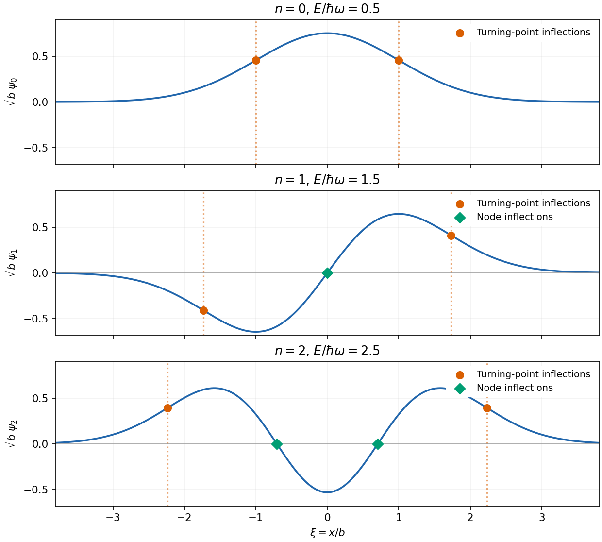
Original lowest harmonic-oscillator wavefunctions with turning-point and node inflections distinguished
. Details. 
Resolving a length requires momentum transfer of order . Taking a hard relativistic scale givesThe full de Broglie wavelength convention gives , differing by ; the intended scale is roughly , far below a proton radius. Two opposing beams have a larger total collision energy, but proton energy is shared among partons: the actual resolution depends on the hard scattering momentum transfer, not simply on beam energy alone.
For radiative temperature uncertainty after background subtraction, write , so and . The two absolute uncertainties are both . If they are independent standard uncertainties,If the percentages instead denote absolute error bounds, linear worst-case propagation gives 0.56%. With correlation coefficient , the standard-uncertainty result is ; subtraction makes positive common errors partly cancel. The independence convention is therefore an assumption, not information supplied by the percentages.
For independent electron arrivals, the shot-noise counting model gives mean transferred charge and count . Poisson statistics implyThis is about 79 electron charges rms. It assumes Poisson shot noise; charge discreteness by itself does not rule out correlations, thermal noise or other apparatus noise.
The canonical commutation relations are , with . Operators from different Cartesian modes commute, so and . Thus is Hermitian and represents an observable on the usual oscillator domain.
Introduce annihilation operators and similarly . Set , and . The Schwinger boson representation givesFor and , and . ThereforeThe two-mode oscillator Casimir identity isSince , , and is conserved. However, is not the zero operator, so there is no general joint eigenbasis. The exception is important: a common eigenstate of two angular-momentum components must satisfy , then the other commutators force . Thus only the sector admits a common state; here that is the oscillator ground state.
Using , with , and selecting the positive energy branch givesEquivalently , so and the degeneracy is , corresponding to .
For observables with finite variances, the Heisenberg uncertainty principle gives ; in particular . It concerns the spreads of measurements in a prepared state, rather than only disturbance by a measuring device. Identical integer-spin particles have symmetric full states and Bose-Einstein statistics; half-integer-spin particles have antisymmetric full states and Fermi-Dirac statistics. The latter imply Pauli exclusion from one complete single-particle state, including spin.
Inside an infinite square well, solutions satisfying both zero boundary conditions arewith zero wavefunction outside. For the ground state, direct integration givesThe infinite-well ground-state uncertainty product follows:The ground state is not a minimum-uncertainty Gaussian. Here momentum variance is the usual kinetic-momentum second moment of the confined state; the hard-wall momentum operator has domain subtleties that do not alter this kinetic-energy result.
For spin degeneracy in filling a one-dimensional well, let and assume the spin levels are degenerate and available. Four spin-zero bosons all occupy the lowest orbital, giving . Four spin- fermions fill two spin states in each of , giving . Spin- fermions have four spin projections, so all four can occupy in different complete states, giving . These fillings do not impose full spin polarization.
matrix multiplication gives , hence . For physical neutron spin, use , so , , and measurement along any axis gives .
For the specified field, . The Time-dependent Schrödinger equation is with . The uniform-field spin precession follows from :
The measurement direction is , as confirmed by the original diagram. Write and . The spinors and have unit norm and inner product . Applying gives eigenvalues and . At they are the usual basis; at they are the basis up to a phase; at the up/down roles are exchanged, with a factor ; and at both return with a minus sign. A spinor changes sign under a full rotation, while its isolated-state measurement probabilities are unchanged.
For spin measurement in the yz plane, projection givesFor these are ; for both are at all times; for they are exchanged; and for they are the same as at zero angle. The constant probabilities also follow from conservation of .
For the two inline operator labels, (a) has eigenvalue , and (b) has eigenvalue , with and . The subscript distinguishes the magnetic quantum number from the electron mass.
Put and . For the proposed radial shape,The angular-momentum term cancels the inverse-square part. The inverse-radius coefficient vanishes if . ThereforeThis nodeless Coulomb radial eigenstate has principal quantum number , not the complete set of hydrogen radial states. Since the spherical harmonic is normalized, radial normalization requiresup to an arbitrary phase.
For the hydrogen ground-state nuclear-volume probability, use . With ,No numerical proton radius is supplied or required. A sharp proton boundary is an approximation to a charge distribution, and the point-Coulomb potential changes inside an extended proton. Finite proton mass, relativistic and electromagnetic corrections also limit the ideal wavefunction's precision.
Classically the kinetic energy must satisfy . For this demands . The hydrogen ground-state probability beyond the classical turning point isA substantial probability lies beyond the classical turning radius; the bound-state wavefunction decays there rather than vanishing.
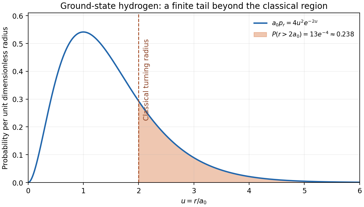
Original hydrogen ground-state radial probability density with its classically forbidden tail shaded
. Details. 
angular momentum generates rotations. Its components obey , and commutes with each component. A compatible basis has and , where . ladder operators change by one, terminate at , and give magnetic substates. Different Cartesian components generally cannot all be sharp simultaneously.
orbital angular momentum is . Its angular eigenfunctions are spherical harmonics, with integer arising from their spatial rotation properties and single-valuedness. spin is intrinsic angular momentum, not literal rotation of a finite charged sphere. It may be half-integer; spin is represented by . For several contributions, obeys the same algebra. Coupling angular momenta permits , with Clebsch-Gordan coefficients relating product and coupled bases. spin-orbit coupling can distinguish these total-angular-momentum sectors.
The Stern-Gerlach apparatus sends a collimated neutral atomic beam through an inhomogeneous magnetic field and records its deflection. A magnetic moment experiences ; field uniformity would produce precession but no analogous net separating force. A classically continuous distribution of moment orientations would broaden the beam continuously. Gerlach and Stern instead observed separated silver-beam components. Reversing or removing the field and comparing the undeflected profile controls the magnetic origin; collimation, velocity spread and finite resolution affect the spots. The original experiment demonstrated space quantization; its modern silver interpretation uses the unpaired electron spin with nearly zero orbital angular momentum, rather than a direct measurement of a free electron's trajectory.[ref]
Der experimentelle Nachweis der Richtungsquantelung im Magnetfeld by Walther Gerlach and Otto Stern. Experimental setup, recorded silver deposits and field-on/off comparison
For two spin- particles, the triplet state sector has and symmetric spin statesThe spin singlet state has and antisymmetric spin stateTheir total values are and zero, while has values and . The singlet is rotationally invariant and gives anticorrelated spin measurements along a common axis. For identical fermions the complete state is antisymmetric: a symmetric spatial state pairs with a singlet spin state, whereas an antisymmetric spatial state pairs with triplet spin. Orbital, spin and coupled angular momenta share an algebra, but their physical origins and allowed representations differ.
In a finite potential barrier with , the stationary Schrödinger equation has exponentially decaying and growing solutions, with local decay constant . Matching the wavefunction and its derivative at finite steps produces a transmitted probability current even though a classical particle at that energy could not cross. energy remains conserved. For a smooth thick barrier, the leading WKB transmission factor isFor a rectangular barrier of height , width and , exact matching gives . Thickness and energy therefore affect transmission exponentially in the opaque limit; prefactors and near-turning-point corrections require more than the leading exponent.
alpha decay illustrates escape from a nuclear well through a Coulomb barrier. A rough decay rate is an internal encounter frequency times barrier penetrability, multiplied by the probability of forming the outgoing cluster; penetrability alone is not a complete nuclear lifetime calculation. In a scanning tunnelling microscope, electron transmission through the vacuum gap gives an approximately exponential distance dependence at fixed conditions. A feedback loop adjusts tip height to maintain current, providing surface information. Bias, tip electronic structure and local electronic density of states also affect the current, so constant-current height is not purely geometric topography. Both applications exploit the same sensitivity of transmission to a classically forbidden region.
The Time-dependent Schrödinger equation governs unitary evolution of a closed system. If is independent of time, expand in its energy eigenstates:An individual energy eigenstate changes only by a phase, so its probability density and time-independent-observable expectations are stationary. Superpositions can have interference terms oscillating at ; fixed energy populations do not imply that every observable is constant.
For general , requires time ordering unless Quantum Hamiltonians at different times commute. The equivalent Heisenberg description evolves observables rather than the state, giving . Explicit time dependence can transfer energy from an applied perturbation.
For a weak perturbation to a known , the first-order transition amplitude from to isIts squared modulus gives the leading transition probability while depletion remains small. A nearly monochromatic perturbation emphasizes energy differences near its quantum of frequency; a continuum and suitable long-time limit yield Fermi's golden rule. These approximations have stated weak-coupling and time-resolution limits; they do not replace exact unitary dynamics in every regime.
For a photon scattering through angle from a free electron initially at rest, conserve energy and momentum. Eliminating the final electron momentum by its relativistic energy relation givesor . The recoil electron gains kinetic energy . The shift is zero forward, one electron Compton wavelength at , and twice that wavelength backward.
Compton's X-ray scattering measurements compared scattered spectra at different angles and identified an angle-dependent shifted component. This supports photon momentum and inelastic recoil, beyond the unchanged-frequency prediction of classical elastic Thomson scattering. Bound electrons and coherent scattering can also produce an unshifted component; initial momentum and binding broaden or modify the ideal free-electron result. Treating an electron as initially free and stationary is therefore a kinematic approximation appropriate when the relevant photon transfer dominates binding scales.[ref]
A Quantum Theory of the Scattering of X-rays by Light Elements by Arthur Holly Compton. Printed pp. 494–495, experimental angular-spectrum comparison; p. 496, recoil discussion
A chi-squared test compares discrepancies with their expected random size. For independent Gaussian observations with known standard deviations, a fitted model givesUnder a correct regular model with fitted parameters, its reference statistical degrees of freedom are usually . Correlated errors instead require with the correct covariance matrix. The reduced statistic has mean about one and standard deviation , so it should not be forced to equal exactly one.
For binned counts, Pearson's statistic is . With a fixed total and populated categories, fitting distribution parameters generally gives . The approximation needs adequately populated expected bins and the appropriate dependence assumptions. Sparse data may require a Poisson likelihood, exact calculation or simulated reference distribution rather than a casual chi-squared approximation.
The upper-tail probability measures how unusual the discrepancy would be under the null model; it is not the probability that the model is true. A large statistic can indicate a wrong model, underestimated noise or unmodelled systematic effects; an unusually small one can indicate overestimated errors or correlations. Residual plots and checks of the noise model are needed alongside the numerical test.
For an experimental-noise interpretation of Nyquist's theorem, a resistor in thermal equilibrium at temperature has one-sided open-circuit voltage-noise spectral densityin the classical range , over an approximately rectangular bandwidth . Across a matched load, half the open-circuit voltage appears, giving available noise power . This is thermal agitation, present without a mean current, and is distinct from shot noise. A real readout weights the spectrum with its transfer function: . Cooling, reduced bandwidth and suitable impedance/noise matching reduce measured noise; the resistor's noise does not simply disappear in an ideal amplifier model.[ref]
Thermal Agitation of Electric Charge in Conductors by Harry Nyquist. Printed p. 113, equations 4–8, thermal emf and bandwidth
The bare name also has a sampling interpretation. The Nyquist–Shannon sampling theorem permits exact reconstruction of a bandlimited signal from sufficiently fast uniform samples. The practical condition is , with an anti-aliasing filter before sampling; otherwise distinct continuous frequencies produce identical samples. Ideal reconstruction uses shifted sinc functions. Critical-rate equality needs an appropriate signal class and can fail for unrestricted edge-frequency sinusoids with unknown phase. Sampling fast enough prevents aliasing, but does not remove thermal noise. This distinction covers the source's unspecified use of “Nyquist's theorem”.[ref]
What the Nyquist Criterion Means to Your Sampled Data System Design by Walt Kester. MT-002, sampled spectra and anti-aliasing discussion
A closed conducting enclosure redistributes surface charge so that an empty interior is protected from an external static electric field. Grounding fixes a reference and drains deposited charge, but an ideal isolated closed conductor also provides inward electrostatic shielding. Real seams, apertures and cables need careful bonding, shielding and feedthrough filtering. For time-varying fields the relevant wavelength, conductivity, geometry and penetration depth matter; a static argument alone is insufficient. Differential wiring and small pickup-loop areas can complement shielding, while careless multiple ground connections create unwanted current loops.
Ordinary copper or aluminium does not generally exclude a static magnetic field. High-permeability shells instead guide magnetic flux around the protected volume. Their effectiveness depends on shape, continuity, openings and saturation; magnetic history and mechanical stress can worsen performance. Nested shields and degaussing can reduce residual fields. Superconducting shielding can exploit the Meissner effect, but trapped flux, openings and critical-field limits require attention.
At nonzero frequency, eddy currents in conducting shields oppose changing magnetic flux. The skin depth isfor a good conductor in the usual diffusion approximation. Thickness of several skin depths suppresses penetration, but the very-low-frequency limit is weak for a normal metal. High-permeability and conducting layers can therefore complement each other. Active compensation coils are an additional method, not passive shielding. Test performance by applying known fields along relevant axes and measuring the residual field or induced signal over the apparatus bandwidth; room-temperature shielding materials and electronics can themselves add noise.
The ideal operational-amplifier rules are zero input currents and, when stable negative feedback maintains unsaturated linear operation, equal input voltages. Infinite open-loop gain motivates the latter; it must not be assumed to guarantee asymptotic stability for every external network.
For the numerical sketch and usefulness discussion, use the transfer function derived in part (c). The chosen values give and . With ,The formal amplitude falls from 5 to zero, with high-frequency slope dB per decade. Its unwrapped phase rises from zero through at to ; the corresponding characteristic frequency is 1.59 kHz. At that frequency the amplitude is 2.5.
These are formal sinusoidal particular-solution curves, not a stable settled filter response. For the formal sinusoidal response of an unstable linear system, replacing by the Laplace variable gives , with a repeated pole at . A homogeneous output contains and grows, so real perturbations lead to supply-limited nonlinear behaviour. With equal positive resistors and capacitors in the frequency-setting network, the general denominator is : the Sallen-Key equal-component stability bound is . For example gives a Butterworth filter response. Thus the Sallen-Key low-pass filter architecture is useful for active filtering with suitable gain and damping, but the stated component set is unsuitable for linear filtering. The component values are retained in this diagnosis.[ref]
Analysis of the Sallen-Key Architecture by James Karki. Sections 3 and 3.4, low-pass transfer function and equal-component gain/Q relation
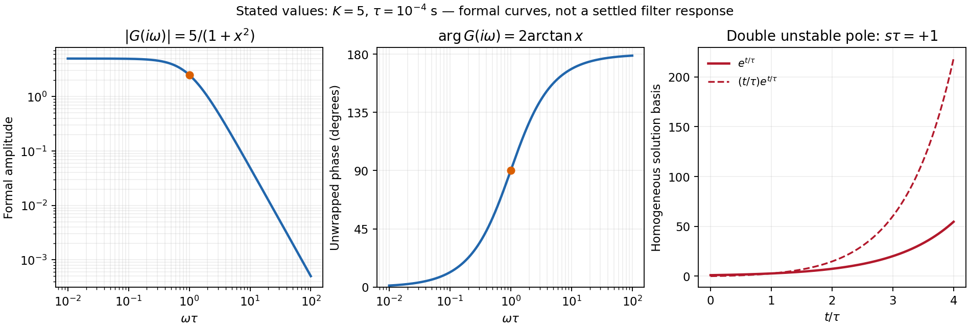
Original formal gain and phase curves for the stated circuit, with its unstable positive Laplace pole explicitly identified
. Details. 
Zero capacitance removes the capacitor branches. No current enters the non-inverting input, so no current flows through or and . The inverting divider gives . Equating the two input voltages in the linear solution gives
Let be the non-inverting input voltage. The feedback divider gives . With , current conservation at this wavefunction node gives , because the amplifier input draws no current. Hence
Current conservation at A, with the capacitor connected from A to the output as verified in the PDF, givesSubstitute and :Therefore, at ,This algebraic transfer function alone does not establish that transients decay; the pole check in the parent solution is necessary for the requested numerical choice.
The Arago spot is a bright axial point inside the geometrical shadow of a circular opaque object. Under coherent illumination, contributions from points around its circular edge have equal optical path to an axial observation point and interfere constructively. It is a Fresnel diffraction effect, so geometrical rays alone miss it. In the ideal paraxial plane-wave model, Babinet's principle gives on axis for disk radius ; thus the axial intensity equals the unobstructed intensity in that model. The whole shadow is not bright: off-axis phases differ and form a localized central feature. Finite source size, poor coherence or an imperfect edge reduce its visibility.
For elliptical polarization from circular and linear components, use coherent waves of the same frequency, propagation direction and fixed relative phase. Let the circular component be and the linear component , with . Their sum has and , soThe tip of the electric field traces an ellipse with unequal semiaxes and . Coherence is necessary: averaging unrelated phases does not create this fixed polarization ellipse.
Reading the time axis, the rapid oscillation has period about , while successive envelope maxima are about apart. The envelope stays nonzero and has a slowly sinusoidal modulation about a positive mean. The corresponding amplitude-modulation model is , with . Product-to-sum givesThus the intended positive-frequency components are , and . The envelope frequency is not itself a separate additive displacement component. These values use the illustrated sinusoidal-modulation interpretation; a finite qualitative trace alone does not uniquely specify every possible spectral component.
At long wavelength, the acoustic phonon branch moves the two atoms in a cell nearly in phase: . In the limit this is rigid translation and . The optical phonon branch moves them oppositely, with stationary cell centre of mass: . Its frequency is finite because adjacent unlike atoms change their separation. For unequal masses the lighter atom has the larger optical displacement. Three-dimensional crystals have three acoustic branches and, with two atoms per primitive cell, three optical branches; longitudinal and transverse directions describe displacement relative to the wavevector. The name optical does not mean that every optical phonon branch is infrared-active: coupling also depends on effective charges and symmetry.
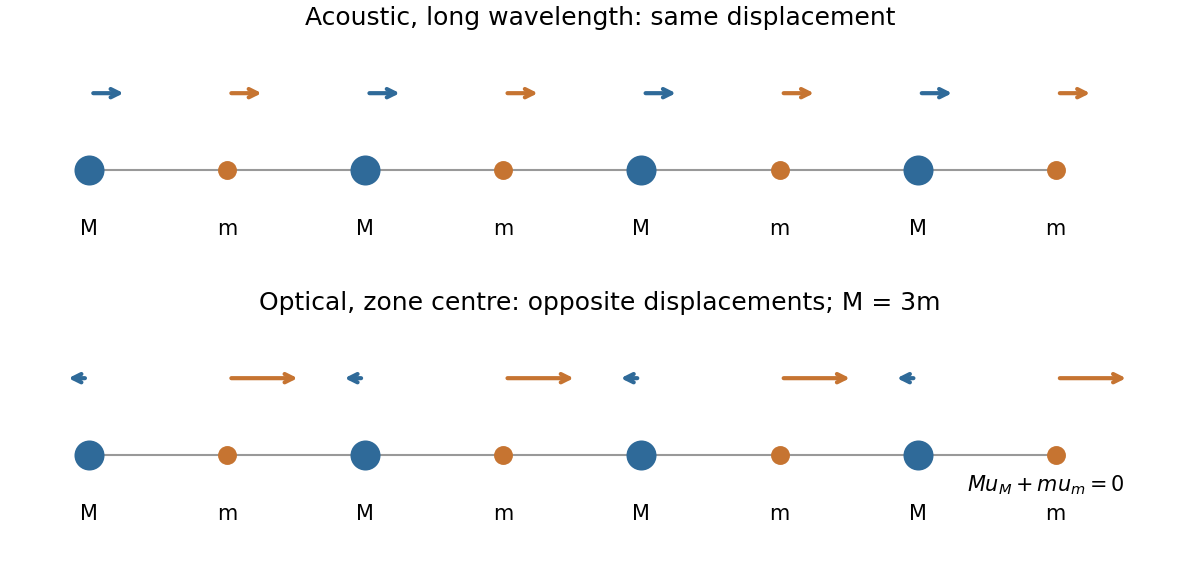
Original long-wavelength acoustic and optical displacement sketches for unequal masses, with optical centre-of-mass cancellation
. Details. 
Let be the number of conduction electrons per atom. Then and the Drude relations give . ConsequentlyUnder an explicit one-electron-per-atom assumption, and . The carrier count is not specified: monatomic does not by itself imply monovalent, so the boxed dependence on is the general result supported by the data. The collision time here is the transport relaxation time inferred within the free-electron model, not a measurement of every microscopic scattering event.
For a narrow packet, phase velocity is and group velocity is . Set . The uncovered surface hasEquality occurs at , also the minimum of . Numerically,The long-wave gravity limit has ; the short-wave capillary limit has .
A compact packet subsequently spreads because different wavenumbers have different group speeds. In the gravity regime , so smaller and longer waves move ahead. Individual crests move twice as fast as the envelope, appearing at its rear and disappearing at its front. In the capillary regime , shorter waves move ahead; the envelope overtakes its slower individual crests, which drift backward relative to it. Thus both the wavelength ordering within the spread packet and the crest motion relative to its envelope reverse.
For the sheet define . The elastic-cover frequency ratio for water waves isAt small , : sheet inertia lowers the frequency, while bending first enters at higher order. At sufficiently large , bending dominates the restoring force and sheet inertia dominates the extra mass, giving . The curve initially dips below one, reaches a minimum, then rises and crosses one. This asymptote describes the supplied ideal dispersion law; arbitrarily large eventually violates a thin-sheet continuum model.
For a pinned-square surface displacement mode, with . The fundamental has . The uncovered frequency is and , soThis uses a square two-dimensional surface mode, not the one-dimensional estimate. A clamped plate or additional hydraulic boundary conditions would require a different mode calculation.
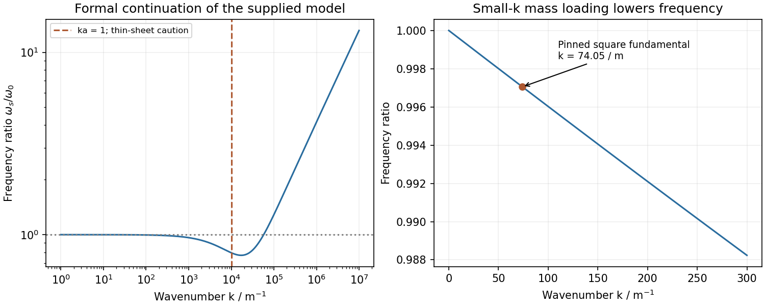
Original sheet-to-uncovered frequency ratio, with the pinned-square fundamental and the ideal large-wavenumber asymptote
. Details. 
The angle in the source ray sketch is inside the gap. Two extra reflections add a full round trip. Comparing adjacent emerging rays on a common outgoing phase plane subtracts the lateral-path contribution, so the optical path difference is , rather than . Thusat transmission maxima. The two internal reflection phases add to an integer full cycle in the stated ideal symmetric-coating model. Snell's law, , converts to the external direction. A fixed internal angle defines a cone and hence an equal-inclination ring in a focal plane.
For identical lossless mirrors the first transmitted amplitude has magnitude times the incident amplitude. Each additional round trip multiplies it by , because is an intensity reflection coefficient for one mirror but the product of the two amplitude reflection magnitudes. Summing the geometric series givesThe maximum is one in this symmetric lossless limit; absorption, unequal mirrors or additional incoherent reflections change it. At fixed angle and negligible material dispersion, and adjacent orders differ by one. For ,
order-safe angular scanning of a Fabry–Pérot spectrum should cover the approximately spectral span within one order while making the instrumental width smaller than . Near normal incidence, requiring the smallest approximate FSR to exceed the span gives , and should exceed roughly . These are design bounds, not a unique optimum. One suitable choice isThe physical spacing is ; an air gap gives . Approximate FSRs near normal incidence are at and at , with widths about and . For a concrete angular scan choose order . The pair lies near internal and the line near ; their widths within this scan remain below . Restricting to this calibrated order window avoids the other-order ring near . Index dispersion and unknown extra source lines would need calibration or order-sorting filters.
The resolving power is approximately : many coherent cavity round trips create a much longer effective optical delay than one traversal. A Michelson instrument with the same available physical delay has less resolving power unless its mirror travel provides a correspondingly long maximum optical path difference. Mirror separation errors spread the round-trip phase; keeping them below a linewidth requires roughlyFor this design the scale is about in an air gap. Both surface flatness and parallelism over the illuminated area, as well as angular collimation and coating uniformity, must support the intended finesse.
The Fraunhofer approximation drops the aperture-dependent quadratic propagation phase. For illuminated extent and observation distance , a sufficient paraxial condition is , with coherent nearly plane incident illumination. Collimation followed by observation in a lens's back focal plane produces the same angular Fourier pattern without an astronomical propagation distance.
Let label the aperture field and let be transverse coordinates of the distant detector, with the axial separation. Expanding the propagation distance retains a common phase and the cross term , while dropping the aperture's quadratic term. Summing the scalar Huygens contributions gives a field proportional to the Fourier transform at . In one dimension, writing , givesRemove the known propagation prefactor and any detector-plane quadratic phase before applying this inverse transform. Recovery needs the complex diffracted field, including phase; its intensity alone is insufficient for this inversion.
The whole-aperture Fraunhofer distance of a coherent array uses the full ten-dish extent, which is about . Thus , and a conventional boundary is about . Far-field propagation must be of order a million kilometres or more, with a stronger inequality for accurate Fraunhofer behaviour. Applying the condition to only one dish or one spacing would miss the array extent.
For equal synchronized dish fields, the array sum is . Its intensity isNear the centre, and the single-dish envelope is nearly constant, giving the requested approximation. A uniformly illuminated circular dish instead supplies the broader envelope , with first zero near . It cannot be ignored over the entire pattern.
Principal array maxima have , height , with spacing approximately arcseconds. There are narrow sidelobes and many grating orders within the dish envelope because . The central maximum's first zeros obey . By reception/transmission reciprocity, the source must therefore move throughfrom zero-order maximum to first minimum. The equatorial geometry fixes the sweep direction; no elapsed time is requested.
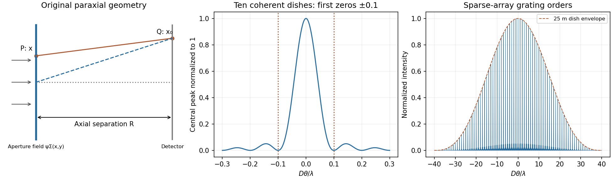
Original labelled Fraunhofer geometry, ten-element central interference lobe and grating orders under a circular-dish envelope
. Details. 
The string speed is . The characteristic impedance is the ratio of the forward-wave transverse force to transverse velocity, . With peak displacement amplitude , the mean power isDisplacement and transverse force are continuous at a massless junction. Since , the displacement amplitudes are and . Taking the incident amplitude real, the light-string motion isIn this standing-and-travelling decomposition of a reflected string wave, the first term travels and the second stands; the decomposition is not a separation into independent incident-power fractions because these fields interfere. The reflected wave has a phase reversal. power coefficients and standing-wave ratio are
For a uniform inserted matching section, unequal exterior impedances require a quarter-wave impedance transformer: and . At equal tension this means middle density and an odd-quarter-wavelength length in that section. Reflections at its two ends then cancel at the design frequency. An arbitrary density or an arbitrary half-wavelength segment cannot perfectly match these unequal exterior strings; the ideal match is frequency-selective.
amplitude scaling along a slowly tapered string instead follows from matching over an adiabatic frequency range. The source fixes frequency, while conserved power and the final characteristic impedance determine amplitude. In the heavy string,Its wave speed halves. The no-reflection approximation needs small fractional characteristic impedance change over each local wavelength, rather than length alone for a taper containing abrupt features.
In a periodic crystal potential, atomic levels broaden into bands of allowed bloch states. Coupling between states of the same symmetry opens avoided crossings, including Bragg-coupled states in the nearly free-electron picture. Bonding and antibonding combinations provide a complementary tight-binding picture. A semiconductor has a filled valence band and an empty conduction band at zero temperature separated by a forbidden energy interval; thermal excitation, light and doping provide mobile electrons and holes. The gap depends on the crystal's periodic potential, bonding and symmetry, not on a classical collision barrier. In a direct gap, the relevant extrema coincide in wavevector.
For the stated parabolic edges, take and . Negligible photon momentum and no phonon make the transition nearly vertical in versus . parabolic-band optical energy sharing divides the excess photon energy in inverse proportion to the effective masses:Thus the initial and final electron energies, relative to the valence-band maximum, areTheir difference is . The selected is about ; either sign gives the same energy in this symmetric approximation.
A shallow donor supplies an electron in a screened impurity potential, so its localized level lies just below the conduction edge. A shallow acceptor binds a hole and has an electron-occupation level just above the valence edge; thermal ionization supplies mobile holes. The level positions are measured relative to the relevant band edge, and deep impurities need not obey this hydrogenic approximation.
For the supplied bound-carrier mass and unit effective ionic charge, dielectric screening and effective mass change the hydrogen binding energy toThis corresponds to and an effective Bohr radius about . The binding is shallow compared with the band gap and typical atomic binding. Trivalent denotes chemical valence, not an unscreened hydrogenic charge of three. An acceptor physically binds a hole; the question's stated is used as its stipulated bound-carrier mass rather than silently replacing it by the separate band-edge .
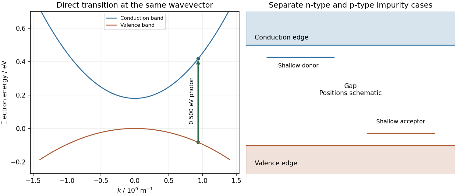
Original direct-gap vertical transition with mass-dependent energy sharing, and separate schematic shallow donor and acceptor levels
. Details. 
With periodic boundary conditions, each state occupies volume and has two spin states. Filling a sphere gives andHere is density of states per volume and per energy; the extensive is . Both spin states are already included.
For divalent magnesium, , givingAt , only electrons within about of the Fermi surface change occupancy. The Sommerfeld heat capacity isEquivalently , with in kelvin, so at room temperature it is about . A temperature was not specified for the estimate; the linear coefficient is the general result.
At sufficiently low temperature, an ordinary nonsuperconducting metal has : electrons dominate at the lowest temperatures, acoustic phonons produce the cubic contribution, and the lattice approaches per mole as temperature exceeds its characteristic Debye scale. Anharmonic expansion can distinguish measured from . In the room-temperature regime, since , so electron excitation is strongly Pauli-limited. The free-electron estimate is only about of the classical lattice scale. Calling it negligible means small relative to the lattice contribution, not identically zero or negligible as . Real band structure and interactions can alter the coefficient.
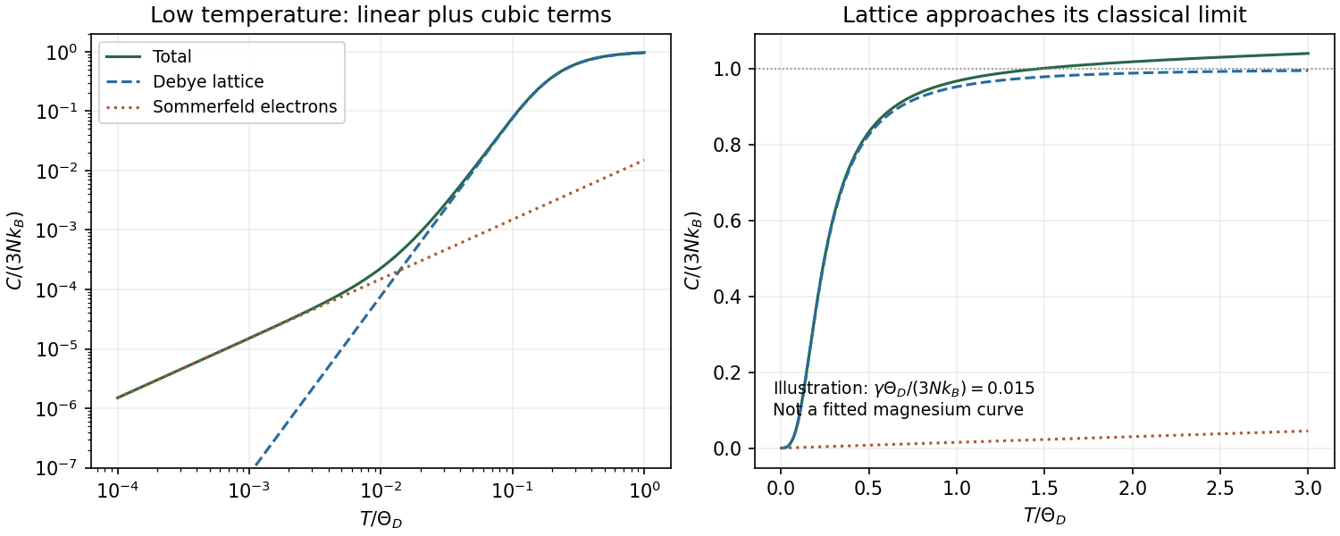
Original illustrative metal heat-capacity regimes: Sommerfeld linear electrons and Debye phonons, with explicit dimensionless model parameters
. Details. 
For , define and . The parameter relating quality factor and viscous damping regimes isAt weak damping it also equals times stored energy divided by energy lost per cycle. The stored-energy convention and frequency matter: this cycle-based interpretation should not be extended to free motions that never complete a cycle.
For the free motion is , where . Thus underdamping means . High gives many oscillations per amplitude-decay time, narrow resonance and strong frequency selectivity; a lightly loaded tuning fork, optical cavity or low-loss electrical resonator provides examples. The amplitude decay time is , while the slowly averaged energy decays with . These times differ by a factor of two.
At critical damping, and , with . There is no ringing; a simple critically damped position indicator can settle without oscillation. For and , there are two real negative decay rates . Increasing very strong drag slows the long-time return, whose rate approaches . A strongly viscously damped mechanical indicator illustrates this regime. These classifications concern the linear homogeneous equation, not every possible nonlinear damping law.
The driven displacement amplitude isThe displacement-resonance threshold of a viscous oscillator requires , or ; it lies at . Some underdamped systems therefore have no such maximum. Average absorbed power instead peaks at for this viscous model. Its half-power frequencies are , so their separation is and . For broad response this ratio remains a useful parameter but not a claim of many free oscillations. The familiar displacement-linewidth version is a high- approximation.
A series RLC circuit has and for the charge oscillation. Resistance dissipates energy, inductance provides the inertial analogue and capacitance the restoring analogue. Ringdown and a calibrated half-power scan independently estimate loss; parasitic resistance, loading and radiation change the measured value. A large increases frequency selectivity but also lengthens settling time, so it is not universally the best instrumental choice.
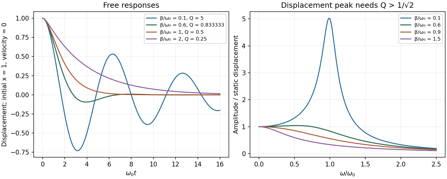
Original free decay and forced-displacement curves distinguishing underdamping, critical damping, overdamping and the resonance threshold
. Details. 
A three-phonon normal process conserves crystal wavevector without a reciprocal-lattice shift, . An Umklapp process instead hasThe crystal can absorb the reciprocal-lattice momentum; after reduction to the first Brillouin zone the phonon drift transporting heat is relaxed. A normal process redistributes phonons while preserving their total crystal momentum, so it is not by itself the same resistive mechanism. energy must also be conserved in either process.
At low temperature, large-wavevector phonons are rare, suppressing Umklapp scattering. Boundary and defect scattering then limit the mean free path; with a nearly constant boundary-limited path, grows as . As temperature increases, heat capacity rises but Umklapp scattering shortens , often producing a electrical conductivity maximum. At sufficiently high temperature a simple anharmonic model has nearly constant and , giving . These are regime estimates, not a universal law for every material or size.
For degenerate carriers with approximately elastic scattering and a common transport relaxation time, and . Using and givesThis is the Wiedemann–Franz law. The same mobile electrons carry charge and heat, but Pauli statistics set the electronic heat capacity and hence the Lorenz number. The relation applies to electronic thermal conductivity, not automatically to total electrical conductivity including phonons. Inelastic electron-phonon scattering can relax energy and charge currents differently; nondegeneracy and strong energy dependence of scattering also limit the simple form.
A meaningful test combines a four-terminal electrical measurement with a steady thermal-gradient measurement on the same sample and temperature range. Contact heat resistance, parasitic heat leaks, phonon conduction and sample geometry must be controlled before interpreting a measured Lorenz ratio as an electronic departure from the law.
A carrier in a locally parabolic isotropic band obeys , soIlluminate a high-mobility crystal with a transverse alternating electric field, sweep a calibrated static magnetic field at known microwave or far-infrared frequency, and detect resonant absorbed power. Cooling lengthens the relaxation time; resolving the resonance generally needs . Varying field direction measures band anisotropy, while circular polarization distinguishes the two senses of rotation for opposite carrier charges. This is orbital motion rather than electron spin resonance.
The classic silicon/germanium measurements used single crystals near , light modulation and circularly polarized microwaves, with directional scans to infer anisotropic carrier-energy surfaces.[ref]
Cyclotron Resonance of Electrons and Holes in Silicon and Germanium Crystals by Gene Dresselhaus and others. Abstract: low-temperature single crystals, light modulation, circular polarization and anisotropy
Carrier generation, calibration, scattering linewidth and inhomogeneity must be separated from a genuine mass shift.In a general band the cyclotron mass is an orbit property, for the appropriate field-normal orbit. It need not equal every component of the band-curvature mass tensor. For an ellipsoidal parabolic band with field along a principal direction it is . Thus a single resonance does not determine a whole effective-mass tensor without angular information.
Articles by others on the same topic
There are currently no matching articles.