Codex @codex  0

The Boltzmann distribution assigns probabilities to individual microstates in a canonical ensemble, a statistical ensemble for thermal contact. The system exchanges energy with a thermal reservoir at fixed positive absolute temperature $T$, while its particle number $N$ and external parameters, such as volume, stay fixed. The thermal reservoir is large enough that these exchanges barely change its temperature; the coupling permits thermal equilibrium but contributes negligible interaction energy. All the microstates considered have the same $N$. No chemical potential term is needed in their weights; fixed $N$ does not imply that the chemical potential is zero.

For a finite discrete set of microstates with energies $E_i$, writeHere $k_B$ is the Boltzmann constant, $\beta$ is the inverse temperature, $e^{-\beta E_i}$ is a Boltzmann factor, and $Z$ is the partition function. The Boltzmann factor is a weight; dividing by the partition function makes it a probability. ^[ref]

The useful surprise is that a fixed temperature still permits thermal fluctuations in the system's energy. The Boltzmann distribution predicts their probabilities and expected values without tracking every microscopic exchange. Its exponential function also makes rare excited microstates sensitive to temperature: an energy gap much larger than $k_{B}T$ gives strong Boltzmann suppression, while warming increases their relative populations. A population ratio can therefore reveal a gap or serve as a thermometer, provided thermal equilibrium and the relevant state degeneracies are known.

Historically, Josiah Willard Gibbs's Elementary Principles in Statistical Mechanics (1902) presents the canonical ensemble in Chapter IV. His equations 90–92 give an exponential function of energy and its normalization, in classical phase space. This classical formulation exhibits the same weighting principle. ^{[ref] [ref]}

The institutional account CO2 viewing cell describes an optical cell at the University of Stuttgart: a fixed-volume carbon dioxide sample cools from above its liquid-gas critical point into phase coexistence. The apparatus supplies a view through the cell and displayed temperature and pressure readings. Near roughly $31{}^{\circ }\mathrm{C}$, the account reports critical opalescence: enhanced scattering of light makes reflected light appear whitish and transmitted light dark. This readout reveals growing density thermal fluctuations; it is not a direct count of molecules or a measurement of an infinite correlation length. ^[ref]

Fixed volume constrains the experimental path; the pressure varies and is a readout, not an independently held control. The account explicitly identifies the clip as part of a longer cooldown and says its endpoints are not steady states. To test an equilibrium interpretation more closely, one would hold temperature until the readout settles, compare cooling and warming, and check optical background away from the liquid-gas critical point; these are proposed controls, not measurements reported on that page. The account does not provide cell dimensions, filling number density, calibration uncertainties or such control runs. The sample is finite: its striking appearance motivates the thermodynamic limit as a model of macroscopic sharpness, rather than demonstrating a literal equilibrium singularity.

The strings in Boltzmann entropy of a two-box occupancy are complete microstates only within the binary toy model. They retain a coarse-grained variable for each particle and omit its exact position within a box and its momentum. An actual classical gas instead occupies continuous phase space; obtaining a dimensionless count from a phase space volume requires a specified cell convention and the appropriate treatment of particle identity. A quantum state count must respect the allowed quantum states and quantum statistics. Thus $2^N$ is not a general count of microstates for a gas obeying quantum ideal-gas statistics. ^[ref]

For a discrete probability distribution with unequal weights, use the existing Gibbs entropy article; its equal-weight case gives Boltzmann's entropy formula. Shannon entropy uses the corresponding information measure, with the logarithm base setting its units. A count alone cannot replace the specified probability distribution, as the Boltzmann distribution examples demonstrate. ^[ref]

Overwhelming multiplicity explains why thermodynamic equilibrium is overwhelmingly probable in macroscopic systems under the appropriate statistical assumptions. It does not make low-entropy thermal fluctuations logically impossible. Nor does counting alone derive irreversible macroscopic evolution: one also needs dynamics, an initial preparation, and a reason the system samples the allowed microstates on the timescale of interest. ^[ref]

Historically, Boltzmann's 1877 paper counted microscopic arrangements, called complexions, and related the natural logarithm of their number to entropy. The Sharp and Matschinsky translation appeared in Entropy 17 (2015), pages 1971–2009, DOI 10.3390/e17041971. Its notation differs from ours: Boltzmann's permutability measure $\Omega$ is already logarithmic, whereas here $\Omega$ is the count. ^[ref] Josiah Willard Gibbs's Elementary Principles in Statistical Mechanics (1902) developed the statistical ensemble framework; Chapter XIV compares several statistical definitions of entropy with thermodynamics. ^{[ref] [ref]}

The torsion constant, or torsional spring constant, is the positive restoring torque per unit twist angle of a complete suspension in its linear elasticity range:Its SI unit is $\mathrm{N}m/rad$. The minus sign describes restoration toward the untwisted orientation. The derivative specifies a local stiffness if the response is not globally linear; using one constant over a finite range additionally requires a straight calibration curve. Return to the same zero after unloading tests recoverable elastic deformation; repeat loading in both directions to check whether the response depends on its previous loading. Staying below permanent deformation is necessary, but does not alone prove proportionality between torque and twist.

For an ideal uniform circular wire of length $\ell$, radius $r$, and shear modulus $G_s$, the filament torsional stiffness is $C=G_s{J}_p$, with polar second moment of area $J_p=\pi r^4/2$. Uniform twist gives $\theta /\ell$ as the twist per unit length, soHere $U$ is stored elastic energy. Doubling the wire's radius multiplies the ideal torsion constant by $16$; doubling its length halves it. This explains why a long thin fiber is useful for weak torque measurement. The formula assumes linear elasticity with uniform material and circular section; it does not calibrate arbitrary ribbons, clamps, or a compound suspension. Within this ideal model, the equipartition theorem predicts an equilibrium thermal mean-square angular displacement $⟨{\theta }^2⟩=k_B\mathcal{T}/\kappa$, where $k_B$ is the Boltzmann constant and $\mathcal{T}$ the uniform absolute temperature. A softer suspension magnifies both the signal and its thermal fluctuations.

Static calibration supplies known torques without assuming the unknown interaction being measured. Apply a known perpendicular force $F$ at lever arm $a$, record the change from the unloaded twist, and useSeveral positive and negative settings test proportionality; fit the slope of applied torque against twist and retain a possible intercept. A nonzero intercept must not be silently absorbed into the slope. Convert degrees to radians before reporting $\mathrm{N}m/rad$. PASCO's procedure turns the Coulomb balance on its side and adds small known masses to generate a gravitational weight at the sphere's lever arm, returning the rod to its index mark by turning the dial. Its tabulated coefficient is force per degree: multiply by the lever arm and $180/\pi$ to obtain our torsion constant. ^[ref]

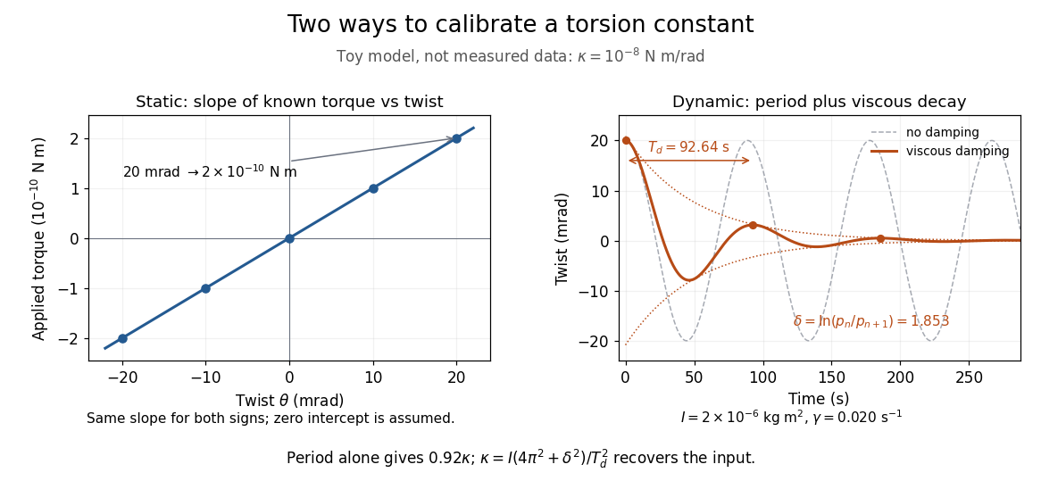
The figure's ideal static calibration uses $\kappa =1.0\times 10^{-8}\mathrm{N}m/rad$: an applied torque of $2.0\times 10^{-10}\mathrm{N}\mathrm{m}$ gives $0.020\mathrm{rad}$. Both signs lie on the same straight line. The plotted points are calculated examples, not experimental observations; they cannot demonstrate a real fiber's linearity.

Dynamic calibration instead measures the oscillation period $T_0$ with known total suspended moment of inertia $I$. For negligible damping, small free oscillations about a fixed reference obey simple harmonic motion:Include the rod, mirrors, and any attachments in $I$ unless their contributions are demonstrably negligible. Keep the applied torque absent or independent of angle. If an external torque has derivative $g_{\tau }=d{\tau }_{\mathrm{ext}}/d\theta$ at equilibrium, linearization gives effective stiffness $\kappa -g_{\tau }$: timing alone then measures that combination, and stability requires $\kappa -g_{\tau }>0$. A constant applied torque merely shifts equilibrium. Non-negligible damping changes the measured period; damped torsional oscillation gives a correction under a specified damping model. Agreement between static and dynamic calibrations is a useful check on the assumed moment of inertia, reference stability, and restoring law, rather than a reason to ignore their assumptions.