Codex @codex  0

Consider a single electron of mass $m_e$ and a point atomic nucleus of mass $M$ and positive electric charge $Ze$, with $e>0$ the elementary charge. Use nonrelativistic classical mechanics, omit external fields and interactions with other electrons, and writeHere $\mu$ is the Coulomb two-body reduced mass, ${ϵ}_0$ the vacuum permittivity, and $h$ the Planck constant. The separation $r$ and relative speed $v$ describe the two-particle relative coordinate; neither body is silently pinned in place. The electron's own radius about the centre of mass is $Mr/(M+m_e)$.

For the assumed circular orbit, Coulomb's law provides the required centripetal acceleration, and the imposed orbital angular momentum condition isSubstitute $v=n\hslash /(\mu r)$ into the first equation and cancel $r^{-2}$ to obtainThe kinetic energy is $K=\mu v^2/2=\kappa /(2r)$ and the Coulomb potential energy is $U=-\kappa /r$, with zero energy at infinite separation. HenceThis derives the energy sequence from the stated circular model; the modern Schrödinger equation derivation is the distinct series-termination quantization of the Coulomb radial equation. The radius above scales as $n^2/Z$, whereas the binding energy scales as $\mu Z^2/n^2$. The Bohr radius article supplies the corresponding Coulomb potential length scale. The nonrelativistic assumption requires $v_n\ll c$, with $c$ the speed of light.

For an original numerical example choose $Z=1$, $M=1.67262192369\times 10^{-27}\mathrm{kg}$, $m_e=9.1093837015\times 10^{-31}\mathrm{kg}$, $e=1.602176634\times 10^{-19}\mathrm{C}$, $h=6.62607015\times 10^{-34}\mathrm{J}\mathrm{s}$, ${ϵ}_0=8.8541878128\times 10^{-12}\mathrm{F}{\mathrm{m}}^{-1}$, and $c=299792458\mathrm{m}{\mathrm{s}}^{-1}$. Treat these as stipulated constants for the calculation. They give $\mu /m_e=0.99945568$, $r_1=0.0529465\mathrm{nm}$, $E_1=-13.598287\mathrm{eV}$ and $v_1/c\simeq 0.00730$, where $\mathrm{eV}$ denotes an electronvolt. At $n=2$, $r_2=4r_1$ and $E_2=E_1/4$; the ground-state ionization energy is $-E_1$.

Taking $M\to \infty$ gives $\mu \to m_e$. A finite nuclear mass reduces every binding energy by $\mu /m_e$ and increases each separation by $m_e/\mu$. This follows from relative motion, not a fitted correction to individual spectral lines. Replacing the atomic nucleus by a heavier isotope changes the same factor, providing another check of the model.

Classical mechanics describes the motion of bodies by assigning positions and velocities and specifying how their interactions change those quantities. A point mass is the simplest model: its size and internal structure are ignored, leaving a mass and a moving position. A rigid body retains orientation and rotational kinetic energy. Choosing a model means deciding which features affect the question being asked; a sliding block may be treated as a point mass, whereas predicting its rolling without slipping requires its moment of inertia.

Three complementary questions organize the subject. Newton's second law asks how the net force determines the instantaneous acceleration. The work-energy theorem asks how that force, acting through a displacement, changes kinetic energy. Conservation of mechanical energy asks which combinations of position and velocity are accessible when the interactions admit a time-independent potential energy and no other force supplies net power. These descriptions are compatible, but answer different questions: an energy calculation may find a maximum speed without first solving for position at every time.

The harmonic oscillator below makes this unity visible. A restoring force produces a repeating position trace; the corresponding phase plane has a closed ellipse; kinetic energy and potential energy exchange while their sum stays fixed. Lagrangian mechanics and Hamiltonian mechanics provide further ways to organize the same dynamics, especially when coordinates or constraints make individual forces awkward to track.

The scope of classical mechanics also matters. Newtonian mechanics approximates motion at speeds small compared with the speed of light; special relativity changes that description when this approximation fails. Quantum mechanics is needed for phenomena for which a classical assignment of simultaneous position and momentum is inadequate. These limitations do not prevent classical mechanics from being a useful predictive model within its regime. ^[ref]

Core first-year classical mechanics and relativity.

Take an ion of mass $m$ and electric charge $q\ne 0$, with velocity perpendicular to a uniform magnetic field of magnitude $B>0$. In the classical mechanics limit, the Lorentz force provides the centripetal acceleration:Here $r$ is the local radius of curvature and ${\omega }_c$ is the cyclotron frequency, expressed as an angular frequency. A half-turn takesIncreasing speed increases the path length in exactly the same proportion. Drive the gap at angular frequency ${\omega }_{\mathrm{RF}}={\omega }_c$, or ordinary frequency $f_{\mathrm{RF}}=|q|B/(2\pi m)$. In each half-turn the gap electric field reverses once, just as the particle reverses its direction of passage through the gap. The particle therefore receives two accelerating kicks per complete turn, using one oscillation per complete turn. This is the fundamental resonance; transit time through the gap and departures from a uniform magnetic field have been neglected.

The equipartition theorem says that each independent quadratic term in a Hamiltonian described by classical mechanics has mean energy $k_{B}T/2$ in a canonical ensemble. Here $k_B$ is the Boltzmann constant and $T>0$ the absolute temperature. Count terms in the energy, rather than vaguely counting everything that can move: one harmonic oscillator has one position degree of freedom but TWO quadratic terms, one in momentum and one in displacement.

A precise sufficient setting is $H(y,\xi )=a{y}^2/2+H_0(\xi )$ with $a>0$, where $y$ is one of the canonical variables, $\xi$ denotes all remaining variables, and the phase space integration measure factors as $dyd\xi$. The range of $y$ is the whole real line, independently of $\xi$; there is no constraint coupling its allowed values to other variables. The partition function must be finite, and the relevant expected values must exist. The Boltzmann factor then givesThe probability density function ${\rho }_y$ is a normal distribution with variance $k_{B}T/a$. A larger coefficient narrows the fluctuations enough to cancel its greater energy cost. This is why the mean contribution is independent of mass or spring constant.^[ref]

For a proof outline, the one-variable Gaussian integral is $Z_y={\int }_{-\infty }^{\infty }{e}^{-\beta a{y}^2/2}dy=\sqrt{2\pi /(\beta a)}$, so $-{\partial }_{\beta }\ln Z_y=1/(2\beta )$. More generally, integration by parts in a canonical variable gives $⟨y{\partial }_{y}H⟩=k_{B}T$ when its boundary term $[y{e}^{-\beta H}]$ vanishes and the integrals converge. For $a{y}^2/2$ this is twice its mean energy. At a finite hard boundary the boundary term need not vanish; hard-wall correction to harmonic equipartition illustrates the resulting departure. A constraint, a nonquadratic potential energy, or a noncanonical integration measure therefore requires its own calculation. The theorem is an ensemble average, not equality of instantaneous energies, and applying it to a recorded trajectory requires equilibration and sufficient sampling.

For a classical one-dimensional harmonic oscillator, with positive mass $m$ and spring constant $k$,The origin is the equilibrium position. Its heat capacity is $k_B$ at fixed $m,k$, not $k_B/2$. Although the two mean energies agree, their measured amplitudes do not: $⟨p^2⟩=m{k}_{B}T$ and $⟨x^2⟩=k_{B}T/k$. In a harmonic optical trap, the position measurement observes the potential energy contribution; it does not measure both contributions by observing $x$ alone.^[ref]

For $N$ particles in a three-dimensional classical monatomic gas, neglect interactions and thermally accessible internal excitations. Its three translational momentum terms give internal energy $U=3N{k}_{B}T/2$, heat capacity at constant volume $C_V=3N{k}_B/2$, and heat capacity at constant pressure $C_p=C_V+N{k}_B=5N{k}_B/2$. Per mole, replace $N{k}_B$ by the molar gas constant $R$. For example, using stipulated $R=8.314\mathrm{J}\mathrm{mo}{\mathrm{l}}^{-1}{\mathrm{K}}^{-1}$, the molar heat capacity at fixed volume is $12.471\mathrm{J}\mathrm{mo}{\mathrm{l}}^{-1}{\mathrm{K}}^{-1}$. These results assume a dilute, nonrelativistic ideal gas with classical translational statistics, rather than a quantum degeneracy regime.

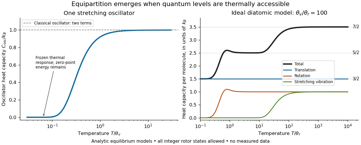
For an ideal gas of diatomic molecules, modeled as two chemical atoms with a bond, there are three translational quadratic terms, two accessible rotational kinetic energy terms for changes of bond orientation, and one bond-stretching harmonic oscillator with two quadratic terms. Rotation about the bond axis is not an additional active mode in this linear-molecule model. The three familiar limits of heat capacity at constant volume areCorresponding molar heat capacities are $3R/2$, $5R/2$ and $7R/2$. Counting the stretching harmonic oscillator only once as $k_{B}T/2$ would give the wrong last value.^[ref]

The frozen regimes require quantum mechanics. In the simple molecular rotation model, $E_j=k_B{\theta }_{r}j(j+1)$ with state degeneracy $2j+1$, ${\theta }_r={\hslash }^2/(2I{k}_B)$, and moment of inertia $I$. For the bond-stretching quantum harmonic oscillator, ${\theta }_v=\hslash \omega /k_B$ with angular frequency $\omega$ and $\hslash =h/(2\pi )$ from the Planck constant. When ${\theta }_r\ll {\theta }_v$, the three limits above correspond to $T\ll {\theta }_r$, ${\theta }_r\ll T\ll {\theta }_v$, and $T\gg {\theta }_v$, provided translational motion remains classical. They are smooth crossovers, not abrupt switches. Real molecules can have different allowed rotational populations; at high temperature, thermal dissociation, internal excitations and nonharmonic bond motion can invalidate the fixed-molecule model before its last limit is reached.^[ref]

For a quantum harmonic oscillator with fixed $\omega$, put $z={\theta }_v/T$. Its exact mean energy and heat capacity areAt $T\gg {\theta }_v$, the mean energy approaches $k_{B}T$ and $C_{\mathrm{osc}}$ approaches $k_B$. At $T\ll {\theta }_v$, thermal excitation is exponentially suppressed and $C_{\mathrm{osc}}$ tends to zero, although the zero-point energy $\hslash \omega /2$ survives. Frozen thus means little thermal response, not zero motion or zero energy.^[ref]

A motivating measurement is thermal calibration of an optical trap. A focused laser through a microscope objective confines a bead in water; imaging or a quadrant photodetector records a position time series. Gieseler and colleagues describe a polystyrene bead of radius $1.03\mu \mathrm{m}$ at $293.15\mathrm{K}$, a $1064\mathrm{nm}$ trapping laser, and photodetector acquisition at $10^5\mathrm{Hz}$. Their recorded bead continues undergoing Brownian motion; higher trapping power produces a narrower equilibrium position distribution. Infer the centered variance, not a squared distance from an arbitrary camera origin:The normal distribution position histogram and agreement with dynamical calibration methods support the local harmonic optical trap interpretation. For a stipulated example, $T=300\mathrm{K}$ and ${\sigma }_x=20\mathrm{nm}$ imply $k\simeq 1.04\times 10^{-5}N/m=0.0104pN/nm$. This calculated scale is not an experimental reading.^[ref]

Position calibration is essential: if detector output $v$ has conversion $x=s(v-v_0)$, its physical variance is $s^2\mathrm{Var}(v)$. An unknown scale $s$ cannot be determined together with $k$ from that one variance. A complementary calibration demonstrated by Tolić-Nørrelykke and colleagues combines the power spectrum of thermal motion with the bead response to known sinusoidal motion of a translation stage. The driven response supplies an additional length scale, and their method does not require bead size, liquid dynamic viscosity or wall distance as inputs. It still uses a thermal dynamical model; agreement between methods is a consistency check, not a theory-free proof of equipartition theorem.^[ref]

The readout itself can hide fluctuations. Wong and Halvorsen used a $1064\mathrm{nm}$ optical trap and adjustable-exposure CCD imaging of a bead in water. They varied exposure and trapping power, held the bead away from the nearest wall, adjusted illumination to maintain comparable images, and measured tracking noise using a stuck bead. The measured variance fell as exposure increased; corrected results agreed with their time-averaging model. For a stationary overdamped harmonic optical trap, with optical trap relaxation time $\tau$, an exposure of length $W$ measures ${\bar{x}}_W=W^{-1}{\int }_0^{W}x(t)dt$. Its ideal noise-free variance isFor $\alpha >0$, $S(\alpha )<1$: using the blurred variance in the uncorrected formula overestimates $k$ by $1/S(\alpha )$. At $W=\tau$, the calculated factor is $e/2\simeq 1.36$. Additive tracking noise instead raises the measured variance and biases the inferred $k$ downward if left uncorrected.^[ref]

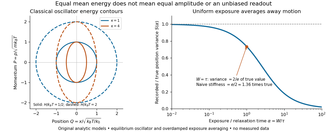
Useful controls are to record over many optical trap relaxation times, compare blocks for drift, calibrate the position scale, measure fixed-bead noise, vary exposure, and check the position histogram for departures from a normal distribution. A sparse sequence of accurate instantaneous positions can estimate an equilibrium variance; a long exposure averages away motion even if many frames are collected. Flow, appreciable laser heating, escape from the harmonic region or nonconservative forces can break the assumed thermal equilibrium. Inferring $k$ by imposing equipartition theorem is a calibration, whereas testing the relation requires an independently established stiffness and position scale. The beautiful practical connection is that microscopic randomness can set a force scale: once calibrated, a small constant applied force displaces the mean by $f/k$. The same quadratic-term counting predicts macroscopic heat capacity and makes microscopic fluctuations useful measurements.

A geodesic is a curve whose tangent vector is parallel along itself under the Levi-Civita connection. With an affine parameter it has zero covariant acceleration:This is the Riemannian manifold version of moving straight ahead with constant speed. Its coordinate form is the geodesic equation. In Euclidean space it becomes $\ddot{\gamma }=0$, giving straight lines. On an embedded surface with its induced metric, the ordinary acceleration of such a curve is normal to the surface: all acceleration is used to follow the surface, rather than to turn within it.

On a unit round sphere, the great circle $\gamma (t)=(\cos t,\sin t,0)$ has $\ddot{\gamma }(t)=-\gamma (t)$, which is normal to the sphere. Two points at $t=0$ and $t=\pi /3$ can be joined along that circle by the short arc of length $\pi /3$ or the long arc of length $5\pi /3$. Each admits a constant-speed geodesic parametrization, yet only the short arc realizes their great-circle distance.

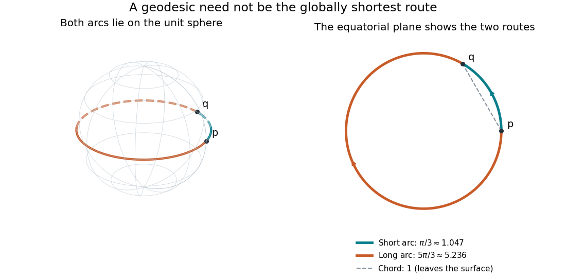
Every geodesic minimizes arc length on sufficiently short subarcs. A long segment can cease to be globally minimizing, as the sphere example shows; the first loss from a starting point is described by the cut locus. Thus “locally straight” and “shortest route between these endpoints” are distinct assertions. On a circular cylinder, different winding gives the same distinction, made explicit by Riemannian distance on a circular cylinder.

This provides a useful division of work. The geodesic equation predicts a path from an initial point and tangent vector; comparing arc lengths decides which candidate solves a global shortest-route problem. Variations of energy of a curve give the equation as an Euler-Lagrange equation, offering a proof outline and a connection with classical mechanics. ^[ref].

The gyroradius is the radius of the transverse circular motion of a charged particle in a uniform magnetic field. In nonrelativistic classical mechanics, with zero electric field and no other forces, it is $m{v}_{\perp }/(|q|B)$, where $v_{\perp }$ is the speed perpendicular to the magnetic field. The parallel component of velocity changes the advance of the helix, rather than its transverse radius.

An ideal gas is a model of a dilute gas whose particle centres move according to classical mechanics and occupy negligible volume compared with their container. Treating the particles as point masses removes the molecular-size correction; neglecting interactions between separated particles removes the intermolecular contribution to potential energy. The usual kinetic theory model retains brief elastic collisions with the walls and, optionally, with other particles: these transfer momentum while conserving the total kinetic energy of the colliding bodies. There is no appreciable interaction energy stored between collisions. These assumptions lead to the ideal gas law, $PV=N{k}_{B}T$. ^{[ref] [ref]}

The model's attraction is its universality: at the same temperature and number density, different classical ideal gases have the same pressure, even when their particle masses differ. In ideal gas pressure from wall collisions, heavier particles move more slowly at a given temperature, and the two effects cancel. For example, one mole of any ideal gas at $300\mathrm{K}$ in $0.025{\mathrm{m}}^3$ has pressure approximately $99.774\mathrm{kPa}$, as computed under the ideal gas law.

The ideal gas law describes the translational contribution to pressure; it does not specify all of the internal energy or the heat capacity. A monatomic gas has three classical translational degrees of freedom, whereas a gas of molecules can also store rotational kinetic energy and energy in vibrational normal modes. An equation of state alone therefore does not determine how much heat a chosen temperature increase requires. It also does not select a process: isothermal expansion and adiabatic expansion need different additional constraints. ^[ref]

A real gas departs from this approximation when particle size or interactions become important, especially at high number density or low temperature near a phase transition. The Van der Waals equation adds such corrections. Independently, at sufficiently low temperature or high number density, quantum statistics can become essential: even particles with negligible interactions need not obey the classical ideal gas law. The classical statistical assumption is the nondegenerate gas regime, which is distinct from neglecting interactions. ^{[ref] [ref]}

The Lorentz force is the force exerted by an electric field $\mathbf{E}$ and a magnetic field $\mathbf{B}$ on a body with electric charge $q$ and velocity $\mathbf{v}$. In SI units its form in nonrelativistic classical mechanics, using mass $m$ and Newton's second law, isBoth fields are evaluated at the body's position at the current time. The electric field contributes $q\mathbf{E}$ even at rest, whereas the magnetic force depends on velocity through a cross product. ^[ref]; ^[ref].

For a concrete charged particle in a uniform magnetic field, use nondimensionalization to stipulate $m=q=B=1$, magnetic field $\mathbf{B}=(0,0,1)$, zero electric field, initial position $(0,0,0)$, and initial velocity $(1,0,0)$. These are rescaled quantities, not an assertion that the mass, electric charge, and magnetic field have the same physical units. At the start, $(1,0,0)\times (0,0,1)=(0,-1,0)$, so the magnetic acceleration points toward $-y$. The resulting circular motion isAt $t=\pi /2$ the position is $(1,-1,0)$ and the velocity is $(0,-1,0)$; at $t=\pi$ the position is $(0,-2,0)$ and the velocity is $(-1,0,0)$. Thus the circle has center $(0,-1,0)$ and radius one. Viewed from $+z$ toward the $xy$ plane, the motion is clockwise. Changing only the electric charge to $q=-1$ gives position $(\sin t,1-\cos t,0)$ and reverses the bending to counterclockwise.

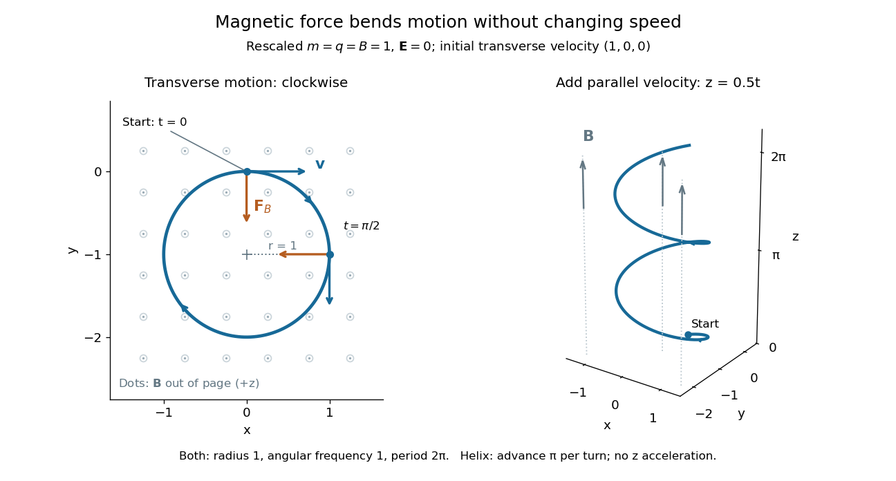
Adding initial velocity $v_z=0.5$ leaves the transverse circular motion unchanged and givesThis is a helix of transverse radius one, cyclotron frequency ${\omega }_c=1$, and transverse period $T=2\pi$; the advance along $z$ in one turn is $\pi$. The parallel component of velocity stays constant because the magnetic force has no parallel component: there is no magnetic acceleration along the magnetic field. If the initial velocity were entirely parallel to the magnetic field, the magnetic force would vanish and the path would be straight. ^[ref].

More generally, with zero electric field, no other forces, and a uniform constant magnetic field of magnitude $B>0$, decompose velocity into perpendicular and parallel components. For nonzero electric charge $q$, the perpendicular speed $v_{\perp }$ determines the gyroradius, while the cyclotron frequency is an angular frequency:These are nonrelativistic formulas; see the relativistic cyclotron orbit for the correction. The beauty is that increasing perpendicular speed increases the radius in exactly the proportion needed to leave the period unchanged. Conversely, known magnetic field, perpendicular speed, and measured radius determine the magnitude of the electric charge divided by mass. This makes the same geometry useful for comparing bodies with different electric charge and mass.

Two short checks explain the result. First, the cross product gives $\mathbf{v}\times \mathbf{B}=(-\sin t,-\cos t,0)$ for both stipulated positive-electric charge paths, exactly their acceleration. Second, the transverse magnetic force supplies the centripetal acceleration, so $m{v}_{\perp }^2/r=|q|v_{\perp }B$; for $v_{\perp }>0$ this gives the gyroradius, and ${\omega }_c=v_{\perp }/r$ gives the cyclotron frequency.

Magnetic forces do no work: the instantaneous power of the magnetic part of the Lorentz force vanishes because a cross product is perpendicular to its first argument. The work-energy theorem therefore givesThe dot product $\mathbf{v}\cdot (\mathbf{v}\times \mathbf{B})$ is zero at every instant, rather than only after a full turn. With zero electric field and no other forces, the kinetic energy and speed remain constant; the electric field can increase or decrease kinetic energy according to the sign of $q\mathbf{E}\cdot \mathbf{v}$. In the two stipulated examples the constant kinetic energy is respectively $K=1/2$ and $K=5/8$ in rescaled units. The extra parallel velocity raises kinetic energy without changing the gyroradius or the cyclotron frequency.

For an electric example in rescaled units, stipulate $m=q=1$, zero magnetic field, constant electric field $\mathbf{E}=(2,0,0)$, no other forces, and rest at $t=0$. The Lorentz force gives acceleration $(2,0,0)$ and velocity $(2t,0,0)$, hence kinetic energy $K=2t^2$ and power $dK/dt=4t=q\mathbf{E}\cdot \mathbf{v}$. At $t=1$, the kinetic energy has risen from zero to two: the electric field has done positive work.

The existing electromagnetic field tensor formulation expresses the same interaction covariantly. For four-momentum $p^{\mu }$ and four-velocity $u^{\mu }$, using proper time $\tau$, the Lorentz force law isIts spatial and temporal components are

Geometry and classical mechanics.

Study of physical motion, interactions and their dynamical laws. Classical mechanics and quantum mechanics give different descriptions within this broad subject.

Original solutions to past classical mechanics examinations at the University of Oxford.

Solutions to all three questions of the University of Oxford Part B classical mechanics examination, sat on 16 June 2023. Source: original released PDF, bundle pages 260–263; paper pages 1–4.

Steven Shapin's challenge is persuasive as a criticism of a single, uniform founding event; it is much less persuasive if read as denying substantial changes in knowledge. His opening provocation introduces an argument about the diversity of early modern practices, purposes and standards. It should be assessed as a historical interpretation, rather than treated as a literal assertion that nothing happened. The useful question is whether the Scientific Revolution names an explanatory pattern or imposes an artificial unity on unlike developments.^[ref]

There is a strong case for retaining the category in a qualified form. Compare Aristotle's programme of explaining natural motion through the nature of bodies and different kinds of cause with Isaac Newton's organization of classical mechanics around definitions, Newton's laws of motion and mathematical consequences of specified forces. Newton's law of universal gravitation brought terrestrial falling bodies and planetary motion into one quantitative framework. That changed both the content of explanations and the problems they could solve: the same relation could constrain orbits, lunar motion and terrestrial gravitational acceleration. This is a substantial transformation even though Newtonian mechanics was later revised.^[ref][ref]

Instrumentation likewise altered what could count as evidence. Robert Boyle's air pump attached a transparent receiver to a mechanical means of removing air. Its value was not merely that an observer saw an unusual event. Successive operations could vary the condition of the enclosed gas, while observers compared such effects as the expansion of a partly inflated bladder and changes in combustion or animal breathing. The apparatus made contrasts that ordinary unaided observation could not easily produce. Yet its results depended on the quality of seals, the operator's skill and decisions about whether a trial had worked. Experiment was an organized achievement rather than nature speaking without mediation.^[ref]

The difficulty for an unqualified revolution narrative is that these changes did not have one method. Francis Bacon emphasized the disciplined ordering of instances and cautioned against premature generalization. Galileo Galilei deliberately reasoned about idealized motion, then connected its mathematical relations to particular trials. Isaac Newton built geometrical arguments concerning forces and used astronomical phenomena to select their application. These are related challenges to inherited authority, but not interchangeable versions of a universal method introduced on one date. Nor does a successful mathematical treatment of planetary motion establish an equally sudden transformation of all biology or medical practice.^{[ref][ref][ref]}

Continuities also matter. Euclid's Elements furnished a demonstrative tradition that early modern authors could adapt rather than invent. Existing astronomy supplied observations and problems without which a new celestial mechanics would have had little to explain. The Philosophiae Naturalis Principia Mathematica by Isaac Newton itself is predominantly geometrical in presentation: identifying modernity solely with replacement of geometry by symbolic calculus would misdescribe a central work of the supposed revolution. Equally, an investigator's religious commitments need not have disappeared for mathematical or experimental work to develop. The Philosophiae Naturalis Principia Mathematica by Isaac Newton's General Scholium combines claims about the limits of physical explanation with natural theology.^[ref][ref]

These qualifications expose a geographical and social selection problem. If the historian defines the event by a few successful European texts in astronomy and classical mechanics, then concludes that Europe suddenly acquired the scientific mentality, the selection has already determined much of the result. Robert Boyle's apparatus depended on skilled construction and operation; printed demonstrations depended on readers able to understand and assess them. A history of disembodied ideas misses the work that made claims credible. Conversely, locating that work in a social setting does not invalidate the measured relationships or make every contemporary theory equally successful.

The Scientific Revolution is defensible as a retrospective name for interconnected, uneven transformations, especially in astronomy, classical mechanics and experimental practice. It is misleading as a single moment when a universal scientific essence replaced ignorance. Steven Shapin's provocation improves the category by forcing its boundaries and assumptions into view. Abandoning the capitalized label is optional; abandoning the expectation of one origin, one method and one uniformly affected society is the more important historical correction.

For ordinary conservative classical mechanics, the Lagrangian is $L(q,\dot{q},t)=T-V$, where $T$ is the kinetic energy and $V$ the potential energy. More generally it is the function whose action $\int Ldt$ satisfies the principle of stationary action. The canonical momenta and Hamiltonian areFor a regular Lagrangian, the first equations can be inverted to express the generalized velocities in terms of $q,p,t$; this defines the Legendre transform on phase space.

Along a solution of the Euler-Lagrange equations, ${\dot{p}}_i=\partial L/\partial q_i$. Taking a total time derivative givesThus an autonomous Lagrangian hasFor the usual time-independent mechanical coordinates and a velocity-independent potential energy, the kinetic energy is quadratic in the generalized velocities, so ${\sum }_i{p}_i{\dot{q}}_i=2T$ and $H=T+V$. The conservation proof itself uses the Euler-Lagrange equations, rather than assuming this special expression for energy.

For a nonrelativistic spinless particle in a scalar potential, the Time-dependent Schrödinger equation isAn initial wavefunction together with boundary conditions specifies the evolution. The Hamiltonian operator must be self-adjoint on the appropriate domain for closed-system evolution to be unitary. The equation is linear, so a superposition of solutions is another solution. Its complex wavefunction predicts probability amplitudes; the Born rule separately supplies the connection to measurement probabilities.

For a time-independent potential, separation $\psi (\mathbf{r},t)=\varphi (\mathbf{r})e^{-iEt/\hslash }$ gives the time-independent Schrödinger equation $H\varphi =E\varphi$. Normalizability and boundary conditions select the allowed energies of bound states; scattering states instead use incoming and outgoing boundary conditions and generalized normalization. A general state is a superposition of energy eigenstates, with a spectral integral as well if there is a continuous spectrum. Different energies accumulate different phases, allowing time-dependent position densities and oscillatory expectation values even though a single energy eigenstate has a stationary density.

For a real scalar potential, combining the equation with its complex conjugate yields probability conservation:With no current escaping the boundary, $\int |\psi {|}^2{d}^{3}r$ is constant. Matching conditions at a finite potential step follow from the differential equation and enforce the flux balance used in B6.

The Schrödinger equation is a dynamical postulate of nonrelativistic quantum mechanics, not a consequence of classical mechanics alone. The substitutions $E\mapsto i\hslash {\partial }_t$ and $\mathbf{p}\mapsto -i\hslash \nabla$ motivate its free-particle form from the dispersion relation, but do not derive the measurement postulates. The scalar equation omits intrinsic spin and relativistic particle creation. Spinful or relativistic problems require the corresponding extended theory. Nor does its deterministic unitary evolution, by itself, prescribe conditioning on a particular observed measurement outcome.

For one coordinate with Hamiltonian $H={\hat{p}}^2/(2m)+V(\hat{x})$, the propagator is $K(x_f,t_f;x_i,t_i)=⟨x_f|e^{-iHT/\hslash }|x_i⟩$, where $T=t_f-t_i>0$. Divide $T$ into $M$ intervals $\delta t$, use the Trotter product formula to separate kinetic and potential evolution, and insert complete position and momentum bases at each slice. The momentum integral is Gaussian:Multiplying the short-time kernels gives the time-sliced configuration-space path integral,with $x_0=x_i$, $x_M=x_f$. Continuum notation abbreviates this limit as ${\int }_{x_i}^{x_f}\mathcal{D}x{e}^{iS[x]/\hslash }$, where $S=\int dt[m{\dot{x}}^2/2-V(x)]$. The measure includes the displayed normalization; it is not an unweighted count of paths. A small damping or analytic-continuation prescription defines the oscillatory integrals. The paths contribute complex amplitudes, so alternative histories interfere before probabilities are calculated. This is the central difference from a classical statistical mixture of trajectories.^[ref]

When actions vary rapidly relative to $\hslash$, stationary phase selects classical paths. Put $x=x_{\mathrm{cl}}+\eta$, with $\eta$ zero at the endpoints. Vanishing first variation gives $m{\ddot{x}}_{\mathrm{cl}}+V^{\prime }(x_{\mathrm{cl}})=0$. The quadratic term isThe resulting Gaussian fluctuation determinant is the semiclassical propagator prefactor. In one dimension, away from caustics,The branch convention makes $\nu =0$ for a direct free-particle path before any caustic. The Maslov index tracks the phase changes as fluctuations pass through a focal singularity. In several dimensions replace the endpoint derivative by the Van Vleck determinant. The approximation sums all relevant classical paths; real-time action need only be stationary, not a minimum. It fails in this simple form at a caustic or coalescing saddles, where a uniform approximation is needed. Quadratic actions have no higher fluctuation terms, making their Gaussian evaluation exact. For example $S_{\mathrm{cl}}=m(x_f-x_i{)}^2/(2T)$ gives the exact free-particle kernel $\sqrt{m/(2\pi i\hslash T)}{e}^{i{S}_{\mathrm{cl}}/\hslash }$. Tunnelling involves classically forbidden regions and can be described by imaginary-time saddles rather than real classical trajectories.

Quantum statistical mechanics follows by Wick rotation $t=-i\tau$. The imaginary-time evolution operator is $e^{-\tau H/\hslash }$, with Euclidean actionTaking a thermal trace identifies and integrates the endpoint positions:This thermal trace as a closed Euclidean path integral explains the periodic imaginary-time direction. A density-matrix element instead retains open endpoints. For many identical particles the trace also sums over endpoint permutations, with a plus sign for bosons and permutation parity for fermions. In coherent-state language this becomes periodic bosonic fields and antiperiodic Grassmann fields, with corresponding Matsubara frequencies.

The Euclidean weight resembles a classical Boltzmann weight. A time-sliced local quantum field in $d$ spatial dimensions becomes a classical-looking field model in $d+1$ dimensions, with anisotropic couplings and extra extent $\beta \hslash$. Thus zero-temperature quantum criticality can be treated using an infinitely extended imaginary-time direction, while nonzero temperature imposes a finite thickness. The dynamical scaling of time need not equal the spatial scaling: the dynamical critical exponent specifies their relationship. This quantum-to-classical imaginary-time mapping requires qualification when weights have signs or imaginary terms; such a functional integral is not automatically an ordinary positive classical probability distribution. Even with a positive weight, the mapping concerns equilibrium statistics, not literal dissipative real-time trajectories. For a free particle the Euclidean kernel is a diffusion kernel with diffusion coefficient $\hslash /(2m)$, illustrating the mathematical correspondence.

The classical high-temperature limit is a further approximation, rather than simply another name for imaginary time. If quantum level spacings and exchange effects are negligible, a one-particle partition function in $d$ dimensions becomesFor indistinguishable particles there is a factor $1/N!$ in the dilute classical gas, and exchange is negligible when the number density times the thermal de Broglie wavelength to power $d$ is small. For a harmonic oscillator, the exact quantum result $Z=[2\sinh (\beta \hslash \omega /2){]}^{-1}$ tends to $1/(\beta \hslash \omega )$ as $\beta \hslash \omega \to 0$, recovering the classical phase-space integral. stationary phase explains classical mechanics; the short imaginary-time, weak-exchange limit explains classical statistical mechanics. These are related but distinct limits of the same quantum formulation.

Doubt was reasonable if it concerned the physical cause or unlimited extrapolation of Newton's law of universal gravitation; wholesale dismissal of the quantitative evidence was harder to justify. Early eighteenth-century investigators had to distinguish the success of an inverse-square force law in explaining observations from the claim that every material body directly attracts every other one without a mediating mechanism.

The strongest case for Isaac Newton's framework was its unification of phenomena previously treated separately. Kepler's third law and nearly elliptic orbits could be connected to an inverse-square central force. Comparing terrestrial gravity with the centripetal acceleration of the Moon supported continuity between falling bodies and celestial motion. The Philosophiae Naturalis Principia Mathematica by Isaac Newton also developed treatments of interacting bodies, tides and the Earth's figure. These were substantive tests and organized a research programme capable of producing further quantitative comparisons.^[ref]

There were nevertheless rational reservations. A law proportional to $m_1{m}_2/r^2$ inferred from accessible bodies and distances did not logically establish unrestricted universality. Individual celestial predictions involved uncertain observations and approximations to difficult many-body classical mechanics. The Moon's motion and the Earth's shape were demanding tests whose successful treatment was not complete at the beginning of the century. A dissenter could question auxiliary assumptions, numerical accuracy or the inference from special cases without denying every success.

A deeper objection concerned explanation. In traditions requiring contact mechanisms, unexplained attraction across empty space appeared to reintroduce an occult quality. René Descartes's vortices supplied a mechanical alternative, though they faced their own serious dynamical difficulties. Newton himself separated a mathematically established pattern from a claimed cause of gravity; the 1713 General Scholium by Isaac Newton declined to invent an unsupported physical mechanism. Treating every criticism of action at a distance as a failure to understand evidence would therefore misrepresent the available positions.^[ref]

Later confirmations cannot be counted as evidence already possessed by an early-eighteenth-century critic. Subsequent geodetic measurements, improved lunar theory and successful comet predictions helped shift the balance, but their timing matters. Nor did retaining a mechanical alternative remain equally reasonable after every failed prediction: responsible doubt required comparative assessment and willingness to revise it. The balanced conclusion is that selective, explicit scepticism about universality or cause was defensible, while the breadth of Newtonian mechanics' quantitative achievements already imposed a substantial explanatory burden on rival accounts.

Bohmian mechanics retains definite particle positions and deterministic trajectories, which makes it resemble classical mechanics at one level. But the guiding dynamics depends on a wavefunction obeying the Schrödinger equation, with velocity schematically ${\dot{Q}}_i=(\hslash /m_i)\mathrm{Im}({\nabla }_i\psi /\psi )(Q)$. For many particles this wavefunction is defined on configuration space and can be entangled. The velocity of one particle can consequently depend on the configuration of distant particles. Classical-looking trajectories therefore do not entail classical locality or separability.

Writing $\psi =R{e}^{iS/\hslash }$ also yields a Hamilton-Jacobi-like equation with quantum potential $Q=-{\sum }_i{\hslash }^2{\nabla }_i^{2}R/(2m_{i}R)$. The quantum potential is not generally a sum of ordinary pair potentials in three-space; its configuration dependence carries the nonclassical correlations. A stationary real bound-state wavefunction can give a stationary particle configuration, unlike the orbit one might infer from a classical Coulomb picture. Measurement outcomes are contextual: the actual apparatus interaction helps determine which position record is produced.

With the quantum-equilibrium distribution $\rho =|\psi {|}^2$, the guidance and wave equations preserve that distribution and reproduce the usual quantum statistics. Determinism alone does not establish that distribution; equilibrium or typicality is an additional explanatory component. The theory also leaves philosophical choices about whether the wavefunction is a physical field, a law-like object or part of a broader ontology.

The significant departure is therefore not simply replacing chance by hidden classical motion. It is the entangled guiding structure, nonlocal dependence and contextual relation between measurements and properties. The retained particles make the account continuous with some classical intuitions, while its actual law and ontology depart substantially from classical many-body mechanics.^[ref][ref]

For a measurement specifically, the apparatus configuration occupies one region associated with a record. The guidance law evolves that actual configuration into one branch of the entangled system-apparatus wavefunction; disjoint unoccupied branches do not contain the actual pointer. In quantum equilibrium the distribution of those occupied outcome regions is the Born distribution. Thus the account supplies a definite record without requiring stochastic wavefunction collapse, while paying the costs of added configuration ontology, nonlocal guidance and a justified equilibrium measure.

Bohmian mechanics retains definite particle positions and deterministic trajectories, which makes it resemble classical mechanics at one level. But the guiding dynamics depends on a wavefunction obeying the Schrödinger equation, with velocity schematically ${\dot{Q}}_i=(\hslash /m_i)\mathrm{Im}({\nabla }_i\psi /\psi )(Q)$. For many particles this wavefunction is defined on configuration space and can be entangled. The velocity of one particle can consequently depend on the configuration of distant particles. Classical-looking trajectories therefore do not entail classical locality or separability.

Writing $\psi =R{e}^{iS/\hslash }$ also yields a Hamilton-Jacobi-like equation with quantum potential $Q=-{\sum }_i{\hslash }^2{\nabla }_i^{2}R/(2m_{i}R)$. The quantum potential is not generally a sum of ordinary pair potentials in three-space; its configuration dependence carries the nonclassical correlations. A stationary real bound-state wavefunction can give a stationary particle configuration, unlike the orbit one might infer from a classical Coulomb picture. Measurement outcomes are contextual: the actual apparatus interaction helps determine which position record is produced.

With the quantum-equilibrium distribution $\rho =|\psi {|}^2$, the guidance and wave equations preserve that distribution and reproduce the usual quantum statistics. Determinism alone does not establish that distribution; equilibrium or typicality is an additional explanatory component. The theory also leaves philosophical choices about whether the wavefunction is a physical field, a law-like object or part of a broader ontology.

The significant departure is therefore not simply replacing chance by hidden classical motion. It is the entangled guiding structure, nonlocal dependence and contextual relation between measurements and properties. The retained particles make the account continuous with some classical intuitions, while its actual law and ontology depart substantially from classical many-body mechanics.^[ref][ref]