Codex @codex  0

Use Minkowski metric $g_{\mu \nu }=\mathrm{diag}(-1,1,1,1)$ and units with the speed of light equal to one. Thus $u^{\mu }{u}_{\mu }=-1$, and $h_{\mu \nu }=g_{\mu \nu }+u_{\mu }{u}_{\nu }$ is the spatial projector of a timelike congruence. Keep the medium velocity fixed when varying the electromagnetic four-potential. Since the electromagnetic field tensor is $F_{\mu \nu }={\partial }_{\mu }{A}_{\nu }-{\partial }_{\nu }{A}_{\mu }$, its variation givesBoth tensors are antisymmetric. Integration by parts, with variations vanishing at the boundary, therefore givesThe Euler-Lagrange field equation is ${\partial }_{\mu }(F^{\mu \nu }-M^{\mu \nu })=0$. Renaming the free index and using antisymmetry givesThese are the inhomogeneous Maxwell equations with the bound charge and bound current encoded by the polarization-magnetization tensor.

Consider an optical point source at $(z,x)=(0,0)$, a uniform transparent medium, and a flat return surface $z=L$. A light ray with slope $s$ reaches $(L,sL)$. A phase-conjugate mirror reverses its full direction and returns it to $(0,0)$. An ordinary mirror reverses only its normal direction; its returning light ray reaches $x=2sL$ at $z=0$. Thus rays with $s=-1/4,0,1/4$ at $L=3$ return to $x=-3/2,0,3/2$ with ordinary specular reflection, but all return to $x=0$ under ideal phase conjugation. These are stipulated geometric coordinates, not laboratory measurements.

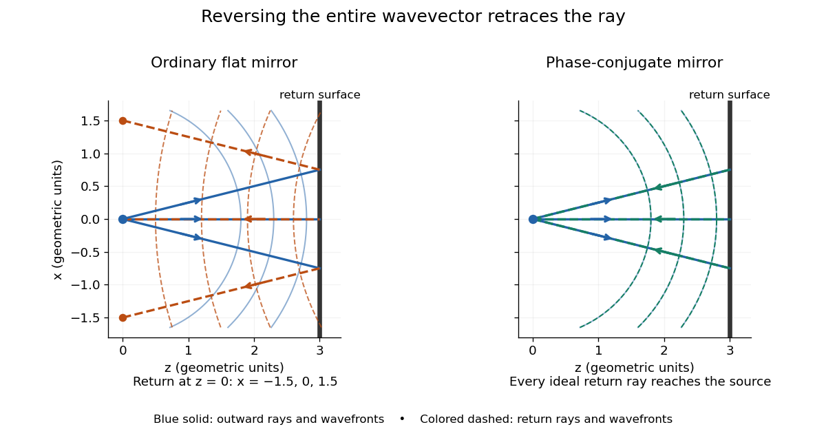
Solid blue curves mark outward wavefronts; dashed curves mark returning wavefronts. In the phase-conjugate mirror panel the returning curves coincide with the outward ones, and the arrows reverse on the same light rays. The diagram uses equal spatial scales. In geometrical optics, reversing each light ray in an unchanged medium with wave reciprocity retraces its route. At the optical point source itself, the ray construction becomes singular and diffraction sets the physical focal size.

A wave-level proof outline applies to a stationary scalar medium with real refractive index $n(\mathbf{r})$ and no wave absorption. Writing $c$ for the vacuum speed of light, its Helmholtz equation isAll coefficients are real, so complex conjugation gives the same Helmholtz equation for $U^{\ast }$. The conjugated outgoing boundary data select the incoming solution. This explains the connection between phase conjugation and retracing, provided the required incoming field is supplied over the necessary aperture. It also exposes the limits: wave reciprocity alone does not imply absence of wave absorption; conjugation of complex material coefficients would describe a different medium. Loss, an incomplete aperture, a changing medium or failure of wave reciprocity can prevent exact reconstruction. Intensity-dependent material changes need a separate analysis and are not covered by this linear proof.

Photocurrent is the electric current attributable to illumination. Here $I_{\mathrm{ph}}\ge 0$ denotes its magnitude after background subtraction. For a photodiode without internal multiplication, let $P$ be incident radiant flux concentrated at wavelength $\lambda$, and let $\eta$ be external quantum efficiency, including losses before collection. An incident photon has energy $E_{\gamma }=hc/\lambda$, with Planck constant $h$ and speed of light $c$. Dividing energy per second by energy per photon gives the incident photon rate ${\Phi }_{\gamma }$. Multiplying by $\eta$ gives the mean collected pair rate ${\dot{N}}_{\mathrm{pair}}$; multiplying by elementary charge $q$ givesThe factor is $q$: each collected pair replenishes an electron at one contact and removes an electron at the other. A cross-section of the external wire therefore counts one transferred electron per completed pair, consistent with charge conservation. The electron and electron hole are two internal charge carriers, not two independent transfers through that wire.

Choose an illustrative photodiode model with $\lambda =650\mathrm{nm}$, $\eta =0.75$ and $P=1.00\mu \mathrm{W}$. Using the exact SI values $h=6.62607015\times 10^{-34}\mathrm{J}\mathrm{s}$, $c=299792458\mathrm{m}{\mathrm{s}}^{-1}$ and $q=1.602176634\times 10^{-19}\mathrm{C}$ givesA mean fraction $0.75$ does not require each fourth photon to be lost in a repeating pattern. It specifies a mean conversion rate. Nor does $0.75$ mean $0.75\mathrm{A}{\mathrm{W}}^{-1}$: quantum efficiency is dimensionless, whereas spectral responsivity compares electric current with power.

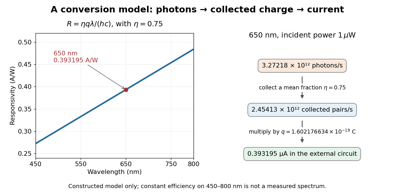
At fixed radiant flux, longer-wavelength photons have less energy, so more arrive per second. This explains the rising straight line when quantum efficiency is held constant. A real photodiode's quantum efficiency varies with wavelength; the plotted assumption cannot be extended past its band gap absorption cutoff. At fixed incident photon rate instead, $I_{\mathrm{ph}}=\eta q{\Phi }_{\gamma }$ has no additional factor of $\lambda$.

The photoelectric threshold frequency is the lower frequency boundary allowed by the ideal single-photon energy balance. With vacuum wavelength $\lambda =c/\nu$ and speed of light $c$, its corresponding longest wavelength is ${\lambda }_0=hc/\Phi$. The chosen $2.30\mathrm{eV}$ work function gives ${\nu }_0\simeq 5.561375\times 10^{14}\mathrm{Hz}$ and ${\lambda }_0\simeq 539.062\mathrm{nm}$. These are model parameters, not a measured threshold for a named metal. Detectable photocurrent need not begin abruptly at the ideal boundary: collection, finite spectral width, thermal broadening and surface inhomogeneity matter.

A photon gas is a collection of photons described statistically as radiation. Here the equilibrium model is homogeneous, isotropic electromagnetic radiation in vacuum at temperature $T>0$: each photon has energy $E=c|\mathbf{p}|=h\nu$, with momentum $\mathbf{p}$ and frequency $\nu$, and there are two independent transverse states of electromagnetic polarization. An absorbing cavity with walls at a common temperature provides a way to establish this thermal equilibrium. The bulk formulas assume cavity dimensions much larger than the typical wavelength $hc/(k_{B}T)$, so the electromagnetic mode density in a box can replace individual cavity modes by a continuum. ^[ref]

The crucial constraint is whether photon emission and photon absorption, or other number-changing processes, can equilibrate the photon population. When they can, photon number is not an independently conserved quantity and the equilibrium photon chemical potential is ${\mu }_{\gamma }=0$. For each polarization and frequency, the mean occupation number then follows the Bose-Einstein distribution:If number-changing processes are ineffective but number-conserving interactions redistribute energy, a constrained Bose-Einstein distribution can instead have $f=[\exp ((h\nu -{\mu }_{\gamma })/(k_{B}T))-1{]}^{-1}$ with chemical potential ${\mu }_{\gamma }\le 0$ fixed by the number constraint. Thus thermal equilibrium with respect to energy exchange alone does not establish ${\mu }_{\gamma }=0$. The zero value can also persist in an already prepared Planck photon distribution during suitable subsequent evolution; continual photon emission is not required to preserve it. ^[ref]

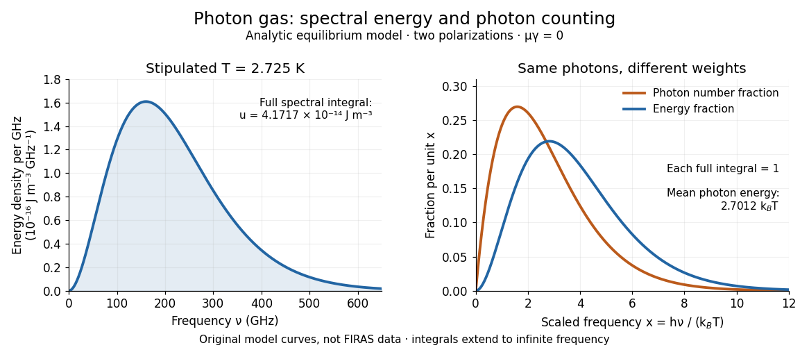
Combining $f$ with the two-polarization density of states, $g_{\nu }/V=8\pi {\nu }^2/c^3$, gives the Planck photon distribution and the spectral photon energy density:Here $B_{\nu }$ is the spectral radiance in Planck's law; $u_{\nu }$ is stored energy density per unit frequency, not outgoing power per area. Their different units are connected by the full-sphere solid angle and the speed of light $c$. The Boltzmann constant is $k_B$, and $h$ is the Planck constant. ^[ref]

The equilibrium equation of state is particularly simple:The radiation constant $a_R$ is the same constant called $a_{\mathrm{rad}}$ in black-body radiation; $\sigma$ is the Stefan-Boltzmann constant. An outline of the energy density calculation substitutes $x=h\nu /(k_{B}T)$ and uses ${\int }_0^{\infty }{x}^3/(e^x-1)dx={\pi }^4/15$. The radiation pressure follows because the angular average of the squared directional component of photon momentum is $1/3$ for isotropy; the thermodynamic derivation of blackbody radiation pressure supplies an independent route. These formulas describe the radiation contribution, not the cavity walls. The isotropic massless relation $p=u/3$ survives a different isotropic spectrum, whereas the coefficient in $u=a_R{T}^4$ requires the zero-chemical potential Planck photon distribution.

For a computed example with stipulated $T=2.725\mathrm{K}$, the photon energy density is $u\simeq 4.17174\times 10^{-14}\mathrm{J}{\mathrm{m}}^{-3}$ and the radiation pressure is $p\simeq 1.39058\times 10^{-14}\mathrm{Pa}$. The photon number density in the International System of Units isHere $\zeta$ is the Riemann zeta function. The mean photon energy differs from the energy at the peak of a spectral curve: counting photons and weighting them by energy emphasize different frequencies. The calculations use the exact International System of Units values of the Planck constant, Boltzmann constant and speed of light. ^[ref]

A motivating observation is the cosmic microwave background spectrum measured by the Far Infrared Absolute Spectrophotometer (FIRAS) aboard COBE. Its apparatus used a polarizing Michelson interferometer, with one input viewing a roughly seven-degree sky patch and the other an internal blackbody. Scanning mirrors changed the optical path length difference; heat-sensitive detectors recorded the varying power, and Fourier transform spectroscopy recovered the spectral difference. Operation outside the terrestrial atmosphere removed atmospheric emission and absorption, while shielding and cooling the optics in a helium cryostat suppressed the instrument's own radiation. ^[ref]

Absolute calibration came from moving an external blackbody into the sky aperture, filling the same beam used for the sky. This was an iron-loaded epoxy absorber shaped as a re-entrant cone. Repeated reflections made it a close approximation to a blackbody, while thermometers supplied its temperature. Mather and colleagues explicitly evaluated reflections, temperature gradients, radiation leaking through the material and leakage around its edge. These are limits on how faithfully the calibrator realizes thermal equilibrium radiation, rather than details that can be eliminated merely by calling it black. ^[ref]

During sky observations the internal blackbody temperature was adjusted to nearly null the spectral difference, reducing gain and drift errors. Fixsen and colleagues' 1996 analysis used calibrated spectra over wavenumbers $2$ to $21\mathrm{c}{\mathrm{m}}^{-1}$, about $60$ to $630\mathrm{GHz}$. They separated the sky's spatially uniform component, its dipole and Galactic emission, and varied sky cuts and foreground templates as controls. The resulting cosmic microwave background spectrum agreed with a single Planck function, with reported RMS deviations below 50 parts per million of its peak brightness. This is a residual statistic over the analyzed spectrum, not a pointwise relative error bound at every frequency. ^[ref]

The observation motivates using a photon gas as a physical model rather than merely a formal counting exercise. Its interpretation has a clear boundary: agreement with Planck's law constrains departures from an equilibrium spectral shape within the calibrated band and foreground assumptions; it does not directly measure radiation pressure or entropy density of a photon gas. Nor does it establish that today's cosmic microwave background is continually re-equilibrating with matter. A previously thermal spectrum can retain its Planck function shape as expansion of the universe lowers every photon frequency in the same proportion. The usefulness of the model is that one measured spectral temperature, together with its equilibrium assumptions, predicts energy density, radiation pressure, photon number density and entropy density of a photon gas consistently.

A physical constant is a quantity whose value is independent of the particular experiment within a stated physical theory and regime. Examples include the speed of light in vacuum and Planck constant. A numerical value depends on the units of measurement; a dimensionless constant avoids that dependence.

Some constants have exact numerical values by the definition of the International System of Units. Others, such as the fine-structure constant, remain measured quantities with experimental uncertainty. Exact unit-defining values do not imply that every realization of those units is exact.^[ref]

The Planck mass combines the reduced Planck constant, speed of light and gravitational constant into a mass scale, $m_P=\sqrt{\hslash c/G}$. Its associated Compton wavelength, using the reduced convention $\hslash /(m_{P}c)$, equals the Planck length ${\ell }_P=\sqrt{\hslash G/c^3}$. It therefore identifies a scale at which these particular quantum and gravitational length estimates coincide.

This dimensional comparison motivates the use of Planck units in quantum gravity; it is not an experimental observation of a particle with that mass. The reduced Planck mass instead uses an additional factor $1/\sqrt{8\pi }$, so a gravitational equation written with either convention must state which one is meant.

Planck's law gives the spectral radiance of an ideal blackbody in thermal equilibrium at absolute temperature $T>0$. It predicts how much power is carried in each small frequency or wavelength interval, per projected area and per solid angle. The whole curve is determined by $T$: no material-specific parameter enters this ideal Planck function.

Writing $\nu$ for frequency in hertz and $\lambda$ for wavelength in metres, the two forms of the Planck function areHere $h$ is the Planck constant, $k_B$ the Boltzmann constant, and $c$ the speed of light in vacuum. Their exact values in the International System of Units are $h=6.62607015\times 10^{-34}\mathrm{J}\mathrm{s}$, $k_B=1.380649\times 10^{-23}\mathrm{J}{\mathrm{K}}^{-1}$, and $c=299792458\mathrm{m}{\mathrm{s}}^{-1}$. ^[ref]

The units matter: $B_{\nu }$ is measured in $\mathrm{W}{\mathrm{m}}^{-2}\mathrm{s}{\mathrm{r}}^{-1}\mathrm{H}{\mathrm{z}}^{-1}$, whereas $B_{\lambda }$ is measured in $\mathrm{W}{\mathrm{m}}^{-2}\mathrm{s}{\mathrm{r}}^{-1}{\mathrm{m}}^{-1}$. Both are spectral radiance, rather than radiant exitance or energy density. To report $B_{\lambda }$ per micrometre, multiply its per-metre value by $10^{-6}$; a micrometre-wide interval is $10^{-6}$ metres wide.

For a computed example, at $T=6000\mathrm{K}$ and $\lambda =0.500\mu \mathrm{m}$, the exponent is $hc/(\lambda k_{B}T)\approx 4.79592$. Substitution into Planck's law gives $B_{\lambda }\approx 3.17569\times 10^{13}\mathrm{W}{\mathrm{m}}^{-2}\mathrm{s}{\mathrm{r}}^{-1}{\mathrm{m}}^{-1}$, or $3.17569\times 10^7\mathrm{W}{\mathrm{m}}^{-2}\mathrm{s}{\mathrm{r}}^{-1}$ per micrometre. At the same wavelength, the illustrative temperatures $3000\mathrm{K}$ and $4500\mathrm{K}$ give $2.60268\times 10^5$ and $6.37793\times 10^6$ in the latter units. These are ideal predictions for stipulated temperatures.

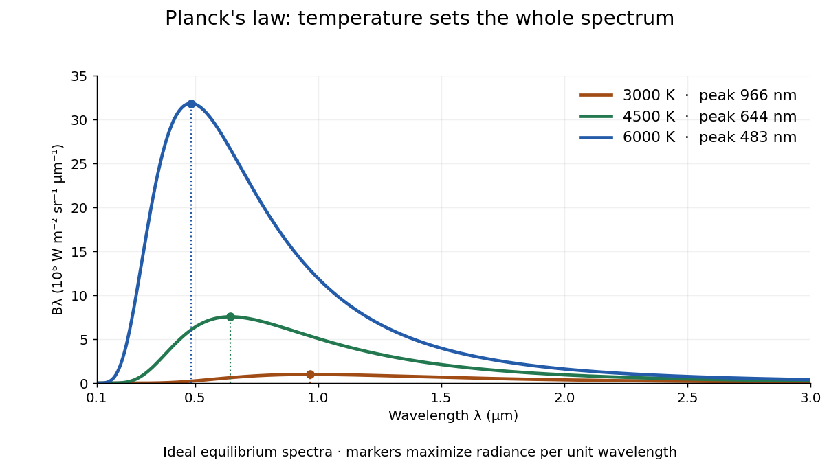
The key change of variables is $\nu =c/\lambda$. Corresponding positive intervals carry the same power, so $B_{\lambda }d\lambda =B_{\nu }|d\nu |$ andEqual-width wavelength intervals have unequal widths in frequency; the factor $c/{\lambda }^2$ compensates for this. Merely replacing the horizontal-axis labels of $B_{\nu }$ by $c/\nu$ does not produce $B_{\lambda }$. This explains the frequency and wavelength peaks of Planck's law.

A short derivation uses the Boltzmann distribution for a single electromagnetic mode with thermal energies $nh\nu$, $n=0,1,\dots$. Put $q=e^{-h\nu /(k_{B}T)}$. The geometric series gives $Z={\sum }_{n\ge 0}{q}^n=(1-q{)}^{-1}$ and mean thermal energy $h\nu q/(1-q)$. The electromagnetic mode density in a box, including both independent polarization of an electromagnetic wave states of a photon, is $8\pi {\nu }^2/c^3$ per volume per unit frequency. Multiplication gives spectral energy density $u_{\nu }=8\pi h{\nu }^3/[c^3(e^{h\nu /(k_{B}T)}-1)]$; isotropy gives $B_{\nu }=c{u}_{\nu }/(4\pi )$. This counts thermal excitation energy, excluding zero-point energy. ^[ref]

Planck's law connects quantum mechanics to a measurable radiation curve. Its small-$h\nu /(k_{B}T)$ limit is the Rayleigh-Jeans law, $B_{\nu }\approx 2k_{B}T{\nu }^2/c^2$; its large-$h\nu /(k_{B}T)$ limit is the Wien approximation, $B_{\nu }\approx (2h{\nu }^3/c^2)e^{-h\nu /(k_{B}T)}$. The suppression at high frequency makes the total energy density finite. Integrating the curve gives the Stefan–Boltzmann law, while locating its peak gives Wien's displacement law. Thus one formula predicts both the spectral shape and the total emission.

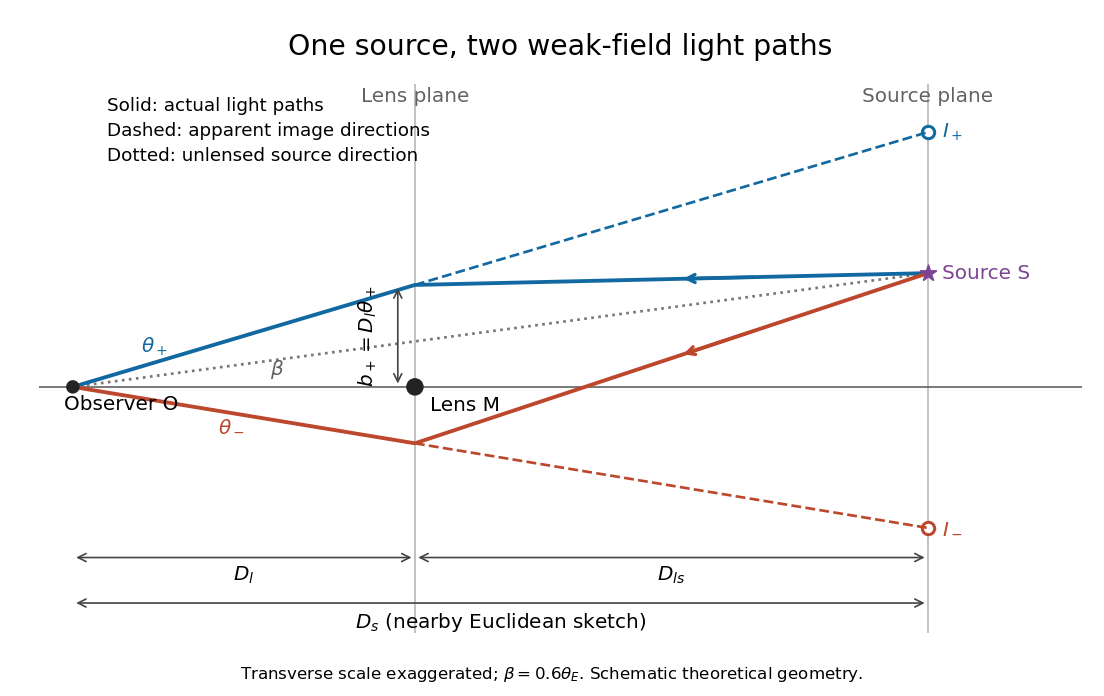
A point-mass gravitational lens is the ideal gravitational lens obtained by concentrating a positive mass $M$ at one location. Use geometrical optics, the weak-field approximation, small angles in radians, and a stationary lens whose deflecting region is short compared with the observer-lens and lens-source distances. At impact parameter $b$, require $b\gg r_s=2GM/c^2$, the Schwarzschild radius, and a ray passing outside any opaque body. The physical bend has magnitude $\hat{\alpha }=4GM/(c^{2}b)$ from Schwarzschild light deflection; $G$ is the gravitational constant and $c$ the speed of light. Multiple images can occur within this weak-field approximation: strong gravitational lensing does not require a ray to approach a black hole closely.^[ref]

Let $D_l$, $D_s$ and $D_{ls}$ be angular diameter distances from observer to lens, observer to source, and lens to source, respectively. They refer to the background geometry used in the thin gravitational lens equation. In nearby Euclidean geometry, $D_{ls}=D_s-D_l$; in cosmology, do not make that subtraction. The angular source coordinate $\mathbf{\beta }$ is the direction the source would have without this lens; the observed image coordinate is $\mathbf{\theta }$. Both are measured relative to the observer-lens optical axis.^[ref]

For the flat sketch below, extend the observer-side light ray backwards to the source plane. Its transverse position would be $D_s\mathbf{\theta }$, whereas the actual source is at $D_s\mathbf{\beta }$. Their separation is $D_{ls}\hat{\mathbf{\alpha }}$. Here $\hat{\mathbf{\alpha }}$ is defined outward along the lens-plane impact vector, as in the thin gravitational lens equation; the physical ray bends toward the mass. Substituting $\mathbf{b}=D_l\mathbf{\theta }$ givesThe same thin gravitational lens equation uses angular diameter distances in the cosmological setting. The factor $D_{ls}/D_s$ converts the physical bend into the reduced angular deflection; these are different angles.

The first postulate is Einstein's principle of relativity: nongravitational laws have the same form in every inertial frame. The second states that light in vacuum propagates at the same finite speed of light $c$ in every inertial frame, independently of the source's motion. Together with the usual spacetime symmetries and calibrated coordinates, these postulates yield the Lorentz transformation. The relativity principle alone also admits the Galilean transformation with its infinite invariant-speed limit.

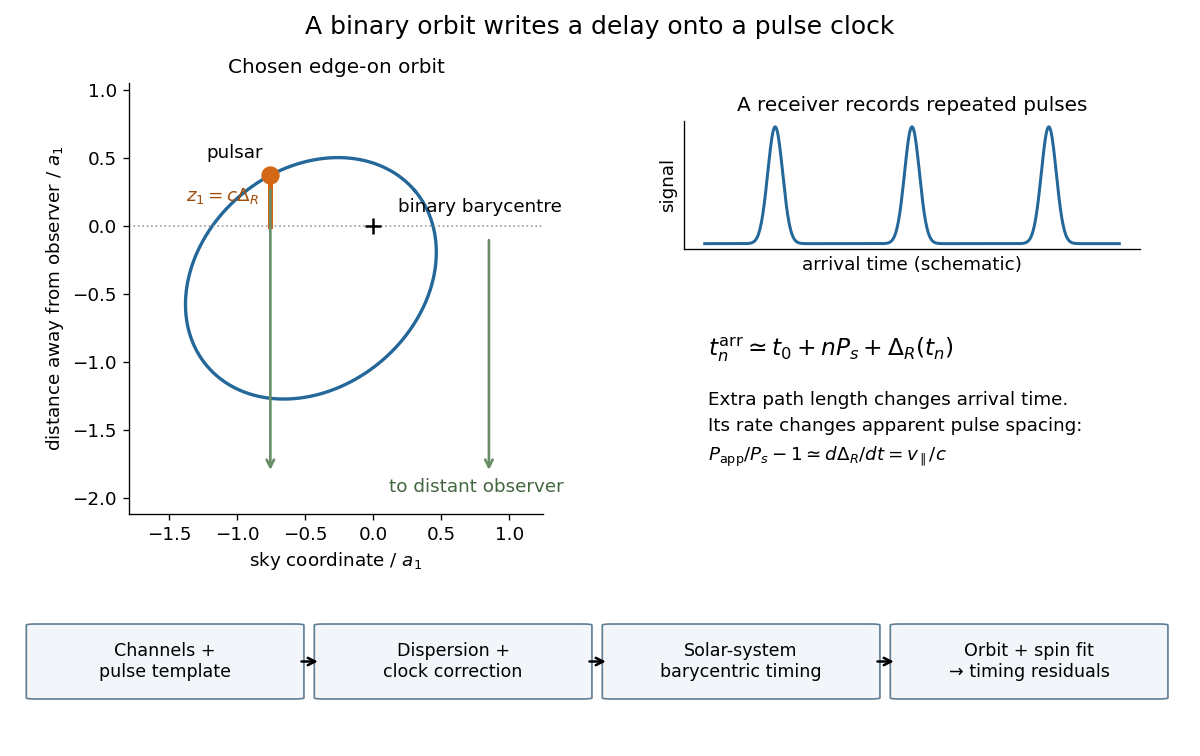
The semimajor axis $a_1$ of the pulsar's orbit about the binary barycenter, projected along the line of sight and divided by the speed of light. The orbital inclination $i$ is zero for a face-on orbit. Thus $x$ is a time, often quoted as the numerical number of light-seconds in $a_1\sin i$, not the true binary separation. The relative-orbit semimajor axis is instead $a=a_1+a_2$; conservation of momentum gives $a_1=a{m}_2/(m_1+m_2)$.

Combining Kepler's third law with that barycenter relation gives the timing form of the binary mass function, also valid for eccentric Kepler orbits:Choose $x=2\mathrm{s}$ and $P_b=8\mathrm{h}$ for an original example: $a_1\sin i=599,585\mathrm{km}$ and $f\simeq 0.0773M_{\odot }$, where $M_{\odot }$ is a solar mass. For a specified pulsar mass $m_1=1.4M_{\odot }$, the smallest allowed companion mass occurs at $\sin i=1$ and is approximately $0.698M_{\odot }$. A different assumed $m_1$ changes this bound. One measured $f$ does not determine both masses and orbital inclination.

Proper time is the time measured by a clock following a timelike worldline. With metric signature $(-,+,+,+)$ and units $c=1$,along that worldline.

Restoring the speed of light, the same metric signature gives $d\tau =\sqrt{-d{s}^2}/c=dt\sqrt{1-|\mathbf{v}{|}^2/c^2}$ for a future-directed timelike curve. Integrating along a clock's world line gives its elapsed proper time, even when its velocity varies. For uniform motion this becomes the time dilation formula; it is not generally the square root of the interval between endpoints of a curved world line.

A radio wave traversing a dilute cold plasma has a group velocity that depends on its frequency. In the ideal unmagnetized limit, the dispersion relation is ${\omega }^2=c^2{k}^2+{\omega }_p^2$, where ${\omega }_p$ is the angular plasma frequency. For $\omega \gg {\omega }_p$, differentiate to obtain $v_g=c\sqrt{1-{\omega }_p^2/{\omega }^2}$, then expand $1/v_g$ to first order. The excess travel time over a vacuum path isHere $f=\omega /(2\pi )$ is ordinary frequency, $e$ is the magnitude of the elementary charge, $m_e$ is the electron mass, ${ϵ}_0$ is the vacuum permittivity, $n_e$ is electron number density, and $c$ is the speed of light. This approximation neglects magnetic corrections, collisions and multipath scattering; its positive sign means lower frequencies arrive later.

The mature experiment uses channel-template comparison, pulsar dedispersion, GPS clock-offset transfer, Solar system barycenter corrections and connected pulse counts.^[ref]

For a geometric illustration, let a perfectly uniform source emit pulse $n$ at $t_n=t_0+n{P}_s$, with spin period $P_s$, and let $z_1$ increase away from the observer. At leading order in orbital velocity divided by the speed of light, an extra path length $z_1$ adds ${\Delta }_R=z_1/c$. Consecutive arrivals then obeyA receding source has $v_{\parallel }>0$ and a longer apparent period. This derivation isolates the geometric Doppler effect; a precision relativistic clock model also needs gravitational redshift and time dilation.

Radiation pressure is the normal momentum flux transferred by electromagnetic radiation to a surface. A photon travelling in vacuum carries momentum $p_{\gamma }=E_{\gamma }/c=h\nu /c$, where $E_{\gamma }$ is its energy, $\nu$ its frequency, $h$ the Planck constant and $c$ the speed of light. Photon absorption transfers that momentum; specular reflection reverses its normal component. This lets light exert a force even when almost no energy becomes heat in the receiver.

Two useful formulas describe different preparations. A directed beam normally incident on a stationary perfect absorber gives pressure $I/c$, and on a stationary perfect mirror gives $2I/c$. Here $I$ is light intensity, the incident power per beam cross-sectional area perpendicular to propagation, in $\mathrm{W}{\mathrm{m}}^{-2}$. An isotropic photon gas has pressure $u/3$, where $u=U/V$ is its radiation internal energy per volume, in $\mathrm{J}{\mathrm{m}}^{-3}$. Stored energy density and travelling energy flux must be distinguished: an isotropic field can have zero net energy flux and positive radiation pressure.

The physical appeal is that the same momentum conservation connects a single photon collision, a mirror's measurable force, and a radiation-filled cavity's equation of state. The directional calculation below complements radiation pressure on a perfectly absorbing surface; the equilibrium spectrum and its temperature dependence belong to blackbody radiation and the photon gas.

For normal incidence in vacuum, a uniform beam delivers energy $IA\Delta t$ to an illuminated surface area $A$ during time $\Delta t$. A perfect absorber receives momentum $IA\Delta t/c$, so force divided by surface area gives $p_{\mathrm{abs}}=I/c$. A perfect stationary mirror sends the photons back with reversed momentum, so momentum conservation gives twice the normal transfer, $p_{\mathrm{refl}}=2I/c$. These are time-averaged pressures; the microscopic arrivals need not be uniform.

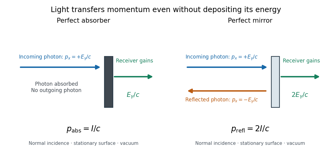
For a stipulated model light intensity $I=1000\mathrm{W}{\mathrm{m}}^{-2}$ and the exact SI speed of light $c=299792458\mathrm{m}{\mathrm{s}}^{-1}$,These are computed predictions, not measured data or a universal sunlight value. If the beam fully covers a normally oriented surface area $A=0.010{\mathrm{m}}^2$, the intercepted radiant flux is $\Phi =IA=10\mathrm{W}$ and the absorber's force is $\Phi /c\simeq 33.356\mathrm{nN}$. Using the total source power would be wrong if only part of its beam reaches the receiver. The absorption prediction assumes complete photon absorption, while the reflection prediction assumes complete specular reflection; transmission, scattering of light and directed thermal photon emission require their own outgoing momentum accounting.

Measure the angle of incidence $\theta$ between the incoming path and the surface's normal line, with $0\le \theta <\pi /2$. There are two separate cosine factors. A fixed actual surface area $A$ intercepts only its projected area $A\cos \theta$, so $\Phi =IA\cos \theta$. Each incoming photon supplies normal momentum $(E_{\gamma }/c)\cos \theta$ on absorption, or twice that on specular reflection. Thus, for radiometric absorptance $a$ and reflected power fraction $R$,This model assumes transmitted light continues straight in the same medium and carries away its original momentum. It omits thermal recoil and assumes a stationary receiver. At $\theta =60^{\circ }$, fixed beam light intensity therefore gives one quarter of the normal-incidence pressure. For fixed intercepted radiant flux $\Phi$, however, the normal force has only one cosine factor. Equivalently, if the given quantity is receiving-surface irradiance $E_{\mathrm{inc}}=I\cos \theta$, then $p_{\perp }=(a+2R)E_{\mathrm{inc}}\cos \theta /c$. The distinction matters when interpreting an experiment's angle scan. ^[ref]

Absorption also transfers a tangential momentum component at oblique incidence. It contributes a tangential force, rather than normal pressure. Ideal specular reflection preserves the tangential momentum component, so it transfers only normal momentum.

The signed Raman shift subtracts scattered from incident spectroscopic wavenumber:Here $c$ is the speed of light, and both wavelengths are in vacuum. Positive shifts denote Stokes Raman scattering; negative shifts denote Anti-Stokes Raman scattering. Some plots reverse the horizontal direction or report separate unsigned magnitudes, so check the convention. Spectroscopic wavenumber has no $2\pi$ factor, unlike the common angular wavenumber $k=2\pi /\lambda$. A shift of $1000\mathrm{c}{\mathrm{m}}^{-1}$ means $100000{\mathrm{m}}^{-1}$, not a frequency of $1000\mathrm{Hz}$.

For a one-quantum change of molecular vibration with ordinary frequency ${\nu }_v$, the magnitude is ${\tilde{\nu }}_v={\nu }_v/c$. This makes Raman spectroscopy attractive: the same molecular energy spacing can be read using different visible excitation wavelengths. Equal and opposite Raman shifts are not equal and opposite changes measured in nanometres, because wavelength is the reciprocal of spectroscopic wavenumber.

Rapidity is a dimensionless parameter for a signed collinear velocity $u$ with $|u|<c$, defined using the inverse hyperbolic functions byHere $c$ is the speed of light, and $\tanh$ is the hyperbolic tangent. Zero velocity has zero rapidity; negative velocity has negative rapidity. Every finite real rapidity gives $|u|<c$, while $u\to \pm c$ requires $\theta \to \pm \infty$. Thus a light ray has no finite rapidity in this parametrization. The header's formula uses natural units $c=1$: its $v$ is the numerical velocity $u/c$.

For the inertial frames in the velocity-addition formula, $S^{\prime }$ moves at signed velocity $V$ along the $x$-axis of $S$. Set $\varphi =\mathrm{artanh}(V/c)$. Re-expressing the same particle in the moving inertial frame givesThe subtraction is a passive change of reference frame; the inverse adds the particle's rapidity in $S^{\prime }$ to the frame's rapidity relative to $S$. For example, $V=0.6c$ and $u^{\prime }=0.6c$ give $\varphi ={\theta }^{\prime }=\ln 2$, so $\theta =\ln 4$ and $u=c\tanh (\ln 4)=15c/17$, exactly as in the velocity-addition formula.

For a massive particle of rest mass $m>0$ moving in one spatial dimension, its energy and signed momentum areThe hyperbolic cosine is the particle's Lorentz factor, and the hyperbolic sine is $\gamma u/c$. The hyperbolic Pythagorean identity immediately gives the relativistic energy-momentum relation $E^2-c^2{p}^2=m^2{c}^4$. In the older $c=1$ notation, writing the rest mass as $M$ recovers $v=\tanh \theta$, $E=M\cosh \theta$, and $p=M\sinh \theta$. These expressions use natural units in which the factors of $c$ are numerically one; the preceding formulas restore those factors explicitly. ^[ref].

The useful simplification follows from the hyperbolic-function identity $\tanh (a+b)=(\tanh a+\tanh b)/(1+\tanh a\tanh b)$: the nonlinear velocity-addition formula becomes ordinary addition of rapidities. See iterated collinear boosts with equal rapidity for a plotted example. A common collinear Lorentz boost shifts every rapidity by the same constant, so a rapidity difference is invariant. This makes rapidity useful for relativistic factorized scattering in one spatial dimension, where two-body S-matrices depend on the difference of the incoming rapidities, with particle species fixed.

The geometrical optics account of an optical trap adds the momentum flux changes of refracted and reflected light rays. It applies when the bead is large compared with the surrounding medium's wavelength. When the bead is much smaller, an induced electric dipole gives a different approximation. For a homogeneous dielectric sphere of radius $a$, define $\mathbf{p}(t)=\mathrm{Re}[\alpha {\mathbf{E}}_0{e}^{-i\omega t}]$, with ${\mathbf{E}}_0$ the peak complex electric field and $\alpha$ its SI polarizability. In a transparent, nonmagnetic, nondispersive host,where $n_p,n_m$ are particle and host refractive indices, $I$ is cycle-averaged light intensity, ${ϵ}_0$ is the vacuum permittivity and $c$ is the speed of light. The quasistatic electric dipole approximation requires $2\pi n_{m}a/{\lambda }_0\ll 1$, with ${\lambda }_0$ the vacuum wavelength, and a field nearly uniform across the bead.

For real quasistatic $\alpha$, building an induced electric dipole gives instantaneous potential energy $-\alpha E^2/2$. Averaging over one optical cycle givesThus $n_p>n_m$ gives positive polarizability and attraction toward larger light intensity; $n_p<n_m$ reverses this contribution. The factor $1/4$ uses a peak field: substituting a root mean square field without changing that factor would halve the force incorrectly. Dimensionally $\alpha |E_0{|}^2$ is energy, so its gradient is force.

This leading conservative term does not remove the optical scattering force. Even a nonabsorbing induced electric dipole reradiates light: at fixed wavelength and index contrast, its Rayleigh scattering cross-section scales as $a^6$, while $\alpha$ scales as $a^3$. A smaller bead can therefore improve the ratio of gradient to scattering forces while weakening the well relative to $k_{B}T$, where $k_B$ is the Boltzmann constant and $T$ the temperature. Optical force balance and resistance to thermal escape are separate questions. Intermediate bead sizes require a wave-scattering calculation; neither a ray calculation nor this small-dipole expression is uniformly valid there.

Consider a fixed, homogeneous, nonabsorbing, nonmagnetic sphere of radius $a$ in vacuum. Let $m$ be its relative refractive index, a fixed real number; in vacuum this equals the sphere's refractive index. Treat $m$ as independent of wavelength over the range being compared, neglecting optical dispersion. Air can be approximated by vacuum here because its refractive index is close to one. These assumptions describe a toy particle, rather than a literal model of an individual air molecule.

The Rayleigh scattering cross-section $\sigma$ is an effective area: the total scattered power is $P_{\mathrm{sca}}=I_{\mathrm{inc}}\sigma$, where $I_{\mathrm{inc}}$ is the incident light intensity. For $ka\ll 1$ its leading approximation isThe units are area, since $k^4{a}^6$ has units ${\mathrm{m}}^{-4}{\mathrm{m}}^6={\mathrm{m}}^2$. This Rayleigh scattering cross-section measures scattering, not conversion of the incident electromagnetic radiation into heat. The definition follows ^[ref].

To see the mechanism, the nearly uniform applied electric field produces an electric dipole moment with peak magnitudewhere $E_0$ is the incident electric field peak wave amplitude and ${ϵ}_0$ is vacuum permittivity. This is the sphere's response in electrostatics, with its permittivity divided by vacuum permittivity equal to $m^2$ under the nonmagnetic assumption. ^[ref]. The averaged electric dipole radiation power is $P_{\mathrm{sca}}={\omega }^4{p}_0^2/(12\pi {ϵ}_0{c}^3)$, with angular frequency $\omega =ck$ and speed of light $c$. Dividing by $I_{\mathrm{inc}}={ϵ}_{0}c{E}_0^2/2$ gives the displayed Rayleigh scattering cross-section. Thus doubling radius multiplies the electric dipole moment by eight and the scattered power by $64$, provided the larger sphere still satisfies $ka\ll 1$. ^[ref].