Random variables are independent when, for every choice of Borel sets ,The requirement covers all these events, not only one selected combination of values. Equivalently, the generated sigma-algebras are independent sigma-algebras, or the joint probability distribution is the product measure of the marginal distributions. For an infinite family, the same condition must hold for every finite subfamily. For random elements, replace Borel sets by measurable sets in their specified target spaces.
For discrete random variables, checking every entry of the joint probability mass function is enough:Summing this identity over the desired sets proves the event formulation. For general real-valued random variables, checking point probabilities alone can say nothing: a pair with no point masses has even when . The all-set definition avoids that trap. See Gautam Iyer, Conditional Probability and Independence, definitions 12, 16 and 18 and proposition 19, with the continuous case treated in his [ref].
For a concrete comparison, let be independent fair bits: each has a Bernoulli distribution with parameter . Their joint probability mass function, with rows and columns , isAll four entries equal the product of the corresponding row and column totals, . For example, : learning one bit leaves the other one's probability distribution unchanged.
Now keep a fair but set . The same marginal distributions give the same product table, yet the actual joint probability mass function isHere differs from , and . Thus matching marginal distributions does not establish independence. Grinstead and Snell formulate the discrete product criterion in Introduction to Probability, section 4.1, definition 4.4, printed page 143.
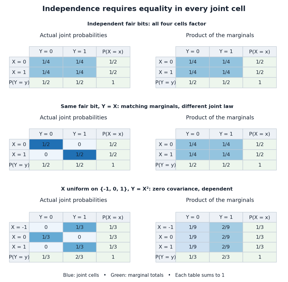
Independence compares every joint probability with the product of the marginals
. Each row compares an actual joint probability mass function with its product of marginal distributions. Marginal totals are shown at the right and bottom of every table; each whole table sums to one. The last example has zero covariance but a visibly different joint table. Details.
Independence is stronger than zero covariance. For square-integrable independent random variables, , so they are uncorrelated random variables. The converse fails: take with a discrete uniform distribution on and . Direct calculation givesNevertheless, is a nonconstant function determined by . The event is exactly the event , so , whereas . The positive and negative contributions to the covariance cancel without erasing the statistical dependence.
The usefulness of independence is that a large joint probability distribution can be assembled from small pieces. For fair independent bits, each of the patterns has probability . Products also simplify expected values, and vanishing cross covariances simplify the variance of a sum. Separate measurable functions of independent random variables remain independent: each output event is already an input event, so the defining product rule still applies. These are consequences of a model's independence assumption; whether the assumption describes actual observations is a question for statistical inference.
Random variables are pairwise independent when every two distinct members are independent random variables. Each pair's joint probability distribution must factor for all its events; examining only a pair's covariance is insufficient. Full independence implies pairwise independence by taking the other sets in the definition to be the whole target spaces. The reverse implication fails once there are three or more variables.
Pairwise independence is enough to add variances: for a finite family of square-integrable pairwise independent random variables,because all cross covariances vanish in the variance of a sum. Thus pairwise independence can support calculations about the size of fluctuations while failing to determine the full joint probability distribution. The following example makes that distinction visible.
Let be independent fair bits, and let be their exclusive or: precisely when . The four possible triples are , each with probability . Each coordinate is a fair bit. Writing out all eight patterns givesEvery pair has all four cells with probability :For , the four allowed triples project to ; for they project to . Each projection lists each pair exactly once, proving pairwise independence. But differs from the product , so the three are not independent random variables. Indeed, any two determine the third. A single coordinate reveals nothing about another, while two coordinates together reveal it completely.
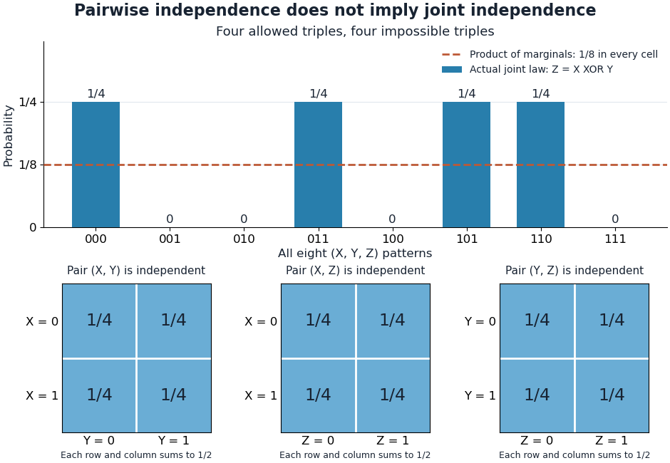
The XOR example hides joint dependence from every pairwise probability table
. The bars show all eight triple patterns against the reference for three independent fair bits. Below, all three pairwise joint probability mass functions have four equal cells of . Details.
The exclusive or example is the complementary-bit version of the two-toss exercise in Grinstead and Snell, Introduction to Probability, section 4.1, exercise 7, printed page 151. It is a compact reason to check the full product rule whenever a calculation uses three-way or higher events.
Random variables and are conditionally independent given when, for every pair of Borel sets , the following identity holds almost surely:Here conditional probabilities are conditional expectations of the corresponding indicator random variables given the sigma-algebra generated by . This defines the condition even when . In terms of regular conditional distributions, the conditional joint law is the product of the conditional marginal distributions for almost every conditioning value.
For discrete random variables, at every with , the condition becomesWhere , this is equivalent to . Once is known, observing provides no further information about .[ref]
Information Theory I — Scene Setting and Statistical Applications (Lecture 9). Information Theory I — Scene Setting and Statistical Applications, Lecture 9, section Conditional independence and conditional mutual information: conditional factorization and predictive irrelevance
For a worked example, suppose a latent variable chooses between two environments with . Given , take to be independent and identically distributed with a Bernoulli distribution of parameter , where and . Think of two separate trials run under the same quiet or active environment. Their conditional joint probability mass functions, with rows and columns , areEach is exactly the product of its own conditional marginal distributions: for , and for . Thus are conditionally independent given .
If the environment is unobserved, the law of total probability averages the two tables:Both unconditional marginal distributions are fair, but . The law of total expectation gives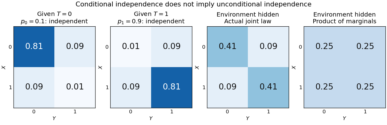
Figure 1.
An unobserved shared environment creates statistical dependence between conditionally independent trials
. The first two tables show independent Bernoulli trials at conditional success probabilities and . Averaging them with equal weights gives the third table. The fourth table is the product of the resulting unconditional marginal distributions, which differs from the actual joint table. These are stipulated model probabilities, not observed frequencies. Details.
Observing makes the active environment more plausible, so it raises to . Knowing the actual environment removes this source of statistical dependence. The covariance induced by a shared latent variable lemma explains the calculation without listing all the outcomes.
This is why conditional independence is useful in statistical modelling: a model can multiply simple conditional laws and then average over a shared latent variable. The resulting observations can remain statistically dependent. Conditional independence graphs organize such information relations; their interpretation as causes requires additional assumptions from causal inference. Conditioning describes the information available to an observer. It does not, by itself, describe what would happen if an experimenter changed a variable.
Return to pairwise independence does not imply joint independence, where are independent fair bits and is their exclusive or. Given , only and remain, each with conditional probability . Given , only and remain, again each with conditional probability . Consequently,The conditional marginal distributions are still fair, so their product has four entries in either case. The actual tables differ: given , and given . Thus unconditional independence need not survive conditioning. Observing whether two bits agree restricts their possible combinations; no physical interaction between the original trials is required to produce that information constraint.
Let be independent random variables, each with a Bernoulli distribution of parameter , and put . Unconditionally, the four ordered pairs each have probability . On the event , only and remain, each with conditional probability . ThusKnowing that exactly one trial succeeded makes observing one outcome informative about the other. This violates conditional independence given , even though the original random variables are independent. Given or , both variables are constant random variables and are conditionally independent there; that does not repair the failure at , an event of positive probability.
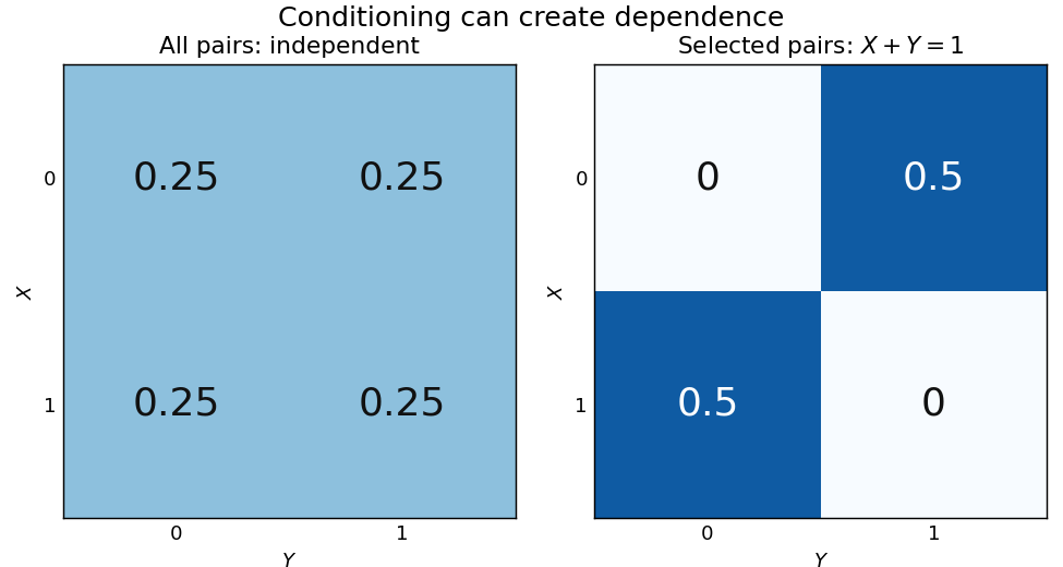
Selecting pairs with exactly one success makes independent trials dependent
. Left: four equally probable outcomes of independent fair Bernoulli trials. The selection retains exactly two pairs. Right: their conditional joint table has zero mass on the diagonal and off it. Within this selected model the conditional covariance is ; the two conditional marginal distributions remain fair. Details.
The conditional covariance here is . Both conditional variances are , so the conditional correlation coefficient is : within the selected group, . These conclusions follow from restricting a finite sample space, without positing any physical interaction between the trials.
This example and the shared-environment example establish both logical directions: independent random variables need not be conditionally independent, and conditionally independent variables need not be independent. When is represented as the joint result of two inputs in a causal directed acyclic graph, conditioning on it has the collider structure associated with collider bias. A probability calculation by itself establishes a dependence relation, not a physical causal mechanism or an intervention.
For a random vector indexed by vertices , its conditional independence graph is the undirected graph with absent exactly when . In a nonsingular multivariate normal distribution, its edges are the nonzero off-diagonal entries of the precision matrix.
Fit the conditional law of each variable given all others and use its predictor support to estimate its neighbours. In a Gaussian graphical model, this is linear regression with coefficients given by conditional regression coefficients from a Gaussian precision matrix. The Nodewise Lasso supplies sparse fits; the OR rule for nodewise graph selection and AND rule for nodewise graph selection combine possibly disagreeing directional supports into an undirected graph.
Minimizing the squared error over each free regression intercept gives the displayed formula. Substitution replaces all data columns by centred columns. The regression intercept is generally not the marginal mean of the response when predictor means are nonzero; the distinction matters in conditional regression coefficients from a Gaussian precision matrix.
The intersection rule retains an edge only when both directions of nodewise regression select it. It is more conservative than the OR rule for nodewise graph selection; the distinction matters because separate finite-sample fits can disagree.
The union rule retains an edge whenever either of the two nodewise regression fits selects the other variable. It is more inclusive than the AND rule for nodewise graph selection and makes an undirected edge decision from potentially asymmetric estimated neighbourhoods.
For a nondegenerate multivariate normal distribution, the conditional independence graph is read from zeros in its precision matrix. Conditional independence of two components given all others is equivalent to a zero cross term in their conditional Gaussian quadratic density, hence to . It does not generally correspond to a zero in the covariance matrix.
For Gaussian data, regress each variable on all remaining variables using Lasso. Nonzero coefficients estimate its neighbours in the conditional independence graph. Symmetrize the separate regressions using either the union or the intersection of their selected directed neighbourhoods.
If D-separation and conditional independence are equivalent for a Directed acyclic graph, its moral graph is its conditional independence graph. After conditioning on all other vertices, an active path can only be a direct edge or a two-edge collider through a common child: two adjacent interior vertices cannot both be colliders. These are exactly the moral edges.
The contraction axiom says thatIt follows directly by multiplying the corresponding conditional-density factorizations.
The decomposition axiom says that implies both and . It follows by marginalizing the joint conditional distribution over the discarded variable.
To test , regress and on and average the products of their residuals. Dividing the scaled average by its empirical second moment produces the generalized covariance measure statistic. Small mean-square nuisance-regression errors and a product-rate condition make it asymptotically pivotal.
If the numerator of the generalized covariance measure statistic obeys a central limit theorem with variance and its empirical residual-product second moment converges in probability to the same positive quantity, the Slutsky theorem makes the studentized statistic converge in distribution to .
If are independent centered square-integrable random variables in a Hilbert space, then for , and hence
An independent and identically distributed sequence combines two conditions: its members are independent random variables, and every member has the same probability distribution. For a finite sequence with common law , this means that for all measurable sets ,For an infinite sequence, require this condition for every finite collection of distinct indices. Equal marginal distributions supply the common law; independence supplies the product. Neither condition supplies the other. Grinstead and Snell call the combination an independent trials process.[ref]
Introduction to Probability by Charles M. Grinstead and J. Laurie Snell. §4.1, Definitions 4.4–4.5, printed pp. 143–144: mutual independence and a common distribution
Choose a Bernoulli distribution with success probability . Four independent draws produce all sixteen binary patterns with probability each. If instead for one fair Bernoulli random variable , every member still has that same Bernoulli distribution, but only patterns
0000 and 1111 occur. Conversely, independently drawn Bernoulli random variables with success probabilities have a product joint probability distribution but unequal marginal distributions.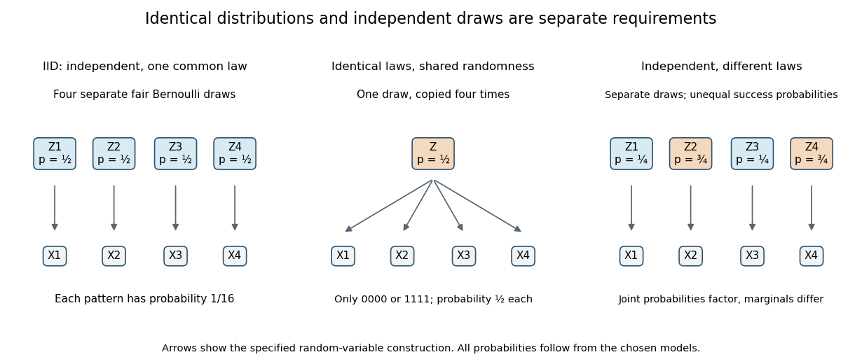
IID sampling combines a common distribution with separate independent draws
. Original constructions of four Bernoulli random variables. Separate arrows in the first and third panels represent explicitly independent source draws; the middle panel copies one shared draw. Dependence and marginal laws are specified by the chosen models. Details.
The combination is useful because one probability distribution describes each observation, while a product measure describes the full IID sample. In particular, an IID sample of finite-variance, real-valued observations has a predictable sample mean: its expected value stays at the population expected value, while its variance of a sample mean decreases as . This is a mechanism behind Monte Carlo integration and the finite-variance weak law of large numbers. Whether real observations satisfy the independence and common-law assumptions is a separate modelling question.
For independent and identically distributed Bernoulli random variables with success probability , the sum has a binomial distribution. Every length- pattern with successes has probability , and the binomial coefficient counts its possible success positions. ThereforeThe usual endpoint convention includes and as deterministic cases. For and , the five probability masses are divided by . The sample mean takes values , with variance and standard deviation . At , its variance is and its standard deviation is .
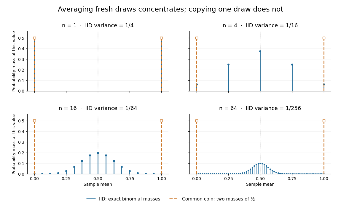
Exact sample-mean distributions distinguish fresh IID draws from a copied common coin
. Original exact binomial distribution probabilities for sample sizes . Blue marks give the mass at each possible mean under independent fair draws. Orange marks give the masses for the same fair draw copied times: at zero and at one for every . These are discrete probability masses, not density values or measured histograms. Details.
In the copied-coin model, for every , so the sample mean is exactly , however large is. Its expected value is and its variance is , matching each observation's marginal variance. The off-diagonal covariances in the variance of a sum explain the difference:For an IID sample, those off-diagonal terms are zero. Repeating the same random input therefore does not create the reduction in fluctuations obtained from fresh independent draws. The general common-plus-individual structure is described by compound-symmetry covariance.
The IID sample property places no integrability condition on its common probability distribution. An IID sample with the standard Cauchy distribution has no finite expected value or variance. The Cauchy sample mean stability result shows that its averages keep that same Cauchy distribution for every sample size. Thus increasing need not concentrate an IID sample around a population mean that does not exist. The finite-variance bound below applies only when its hypotheses hold.
Draw two different labels uniformly from using sampling without replacement. Each position has a uniform distribution on a finite set, but . Two independent random variables with those same marginal distributions would match with probability . Equal marginal laws therefore do not make this sample an IID sample. Mark some of those four labels as successes. Their count in the two draws has a hypergeometric distribution; independent Bernoulli trials with a common success probability give a binomial distribution.
Articles by others on the same topic
There are currently no matching articles.