Codex @codex  0

Osmotic pressure is the excess pressure needed on a chemical solution to maintain osmotic thermodynamic equilibrium with pure solvent across a semipermeable membrane. For a nearly incompressible solvent, equality of chemical potential gives $\Pi \simeq -(RT/{\bar{V}}_w)\ln a_w$. It is an equilibrium property; an observed initial swelling rate is a different measurement.^[ref]

For a dilute ideal chemical solution of retained particles,Here $n$ is the amount of substance of independently dissolved solute particles, measured in moles; $V$ is the final volume of chemical solution, not the starting volume of pure solvent. Count the resulting ions separately if a solute dissociates; do not multiply twice if $n$ already counts them. With $c_{\mathrm{osm}}$ in $\mathrm{mol}{\mathrm{m}}^{-3}$ and $R$ in $\mathrm{J}\mathrm{mo}{\mathrm{l}}^{-1}{\mathrm{K}}^{-1}$, $RT{c}_{\mathrm{osm}}$ has units $\mathrm{J}{\mathrm{m}}^{-3}=\mathrm{Pa}$. This resembles the ideal gas law, although the particles here are dissolved in a liquid.

The assumptions are uniform temperature, a dilute ideal chemical solution, a nearly incompressible solvent, and a semipermeable membrane that retains the counted solutes while passing solvent. Association, incomplete dissociation and interactions change the relation between added material and independent particles; nonideal thermodynamic activities invalidate simple particle counting. The formula does not describe a concentrated brine merely because the apparatus contains a membrane.

A short derivation explains why particles are counted. In an ideal mixture, $a_w=x_w=n_w/(n_w+n)$, with $n_w$ the amount of substance of water. If $n\ll n_w$, then $-\ln x_w=\ln (1+n/n_w)\simeq n/n_w$ and $V\simeq n_w{\bar{V}}_w$. Substitution gives $\Pi \simeq RTn/V$. This is a dilute-limit approximation, not a claim that water molecules stop moving or that dissolved particles are a gas.

Passive transport is net movement down the transported substance's electrochemical gradient without coupling that movement to another source of free energy. Facilitated diffusion is passive transport through an ion channel or a passive carrier protein. Providing such a route can speed passage, but does not turn an uphill transfer into a downhill one. For an uncharged solute under the ideal conditions above, net passive transport runs from higher to lower concentration; for an ion, the membrane potential also matters. See Cooper, The Cell: transport of small molecules.

In the figure, stipulate eight neutral solute tracers in A and two in B, with equal fixed volumes, identical surroundings, and no imposed electric potential difference. The concentration ratio is $c_{\mathrm{A}}/c_{\mathrm{B}}=8/2=4$, so A-to-B transfer has $\Delta \tilde{\mu }=-RT\ln 4\simeq -1.38629RT$, or $-3.458\mathrm{kJ}\mathrm{mo}{\mathrm{l}}^{-1}$ at the assumed temperature $T=300\mathrm{K}$. If this solute can cross, thermodynamic equilibrium has equal expected concentrations: five tracers per side on average. Individual crossings occur in both directions; an observed ten-particle snapshot need not contain exactly five on each side. These stipulated counts illustrate a driving force, not a measured flow rate or a prediction of the time to equilibrate.

For a separate illustrative ion calculation, keep $c_{\mathrm{A}}/c_{\mathrm{B}}=4$, but assign $z=+1$ and $V_{\mathrm{A}}-V_{\mathrm{B}}=-60\mathrm{mV}$ at $300\mathrm{K}$. Using $R\simeq 8.31446\mathrm{J}\mathrm{mo}{\mathrm{l}}^{-1}{\mathrm{K}}^{-1}$ and $F\simeq 96485.33\mathrm{C}\mathrm{mo}{\mathrm{l}}^{-1}$, B-to-A transfer gives $RT\ln 4-0.060F\simeq 3.458-5.789=-2.331\mathrm{kJ}\mathrm{mo}{\mathrm{l}}^{-1}$. Thus an appropriate open ion channel can permit passive transport toward the higher concentration: the electrical contribution outweighs the opposing chemical potential contribution. This stipulated membrane potential is not inferred from the tracer counts.

At a common membrane voltage, an ion is in electrochemical equilibrium only if its own Nernst potential equals that voltage. The four independently calculated equilibrium voltages areThus at $V_m=-90$ mV only chloride is at its listed equilibrium voltage. Potassium has an outward positive-current driving voltage $V_m-E_K=+7.74$ mV. Sodium and calcium have negative driving voltages, $-156.60$ and $-220$ mV respectively, favoring inward positive-ion movement when their channels are open. Chloride has zero net electrochemical drive under these ideal conditions.

A resting potential is not a claim that every permeant chemical species is in thermodynamic equilibrium. A membrane with several electrical conductances can have zero total electric current even though individual ionic electric currents flow and cancel. Pumps maintain the concentration differences by consuming Gibbs free energy. Conversely, a closed channel can prevent substantial ion flux even when the ion's electrochemical potential difference is nonzero: absence of flux due to impermeability is not the same as electrochemical equilibrium. The listed concentrations could not all be passive equilibrium distributions at one voltage because their Nernst potentials differ.

Detailed balance means that at thermodynamic equilibrium each elementary transition and its reverse carry equal probability flux. For normalized state probabilities $A_{\mathrm{eq}}$ and $B_{\mathrm{eq}}$,With the printed convention $\Delta G_{AB}=G_A-G_B$, the sign is thereforeThe $G$ values are free energies per system, including internal degeneracies; for molar Gibbs free energies, replace $k_{B}T$ by $RT$. If B has lower free energy, its forward-to-reverse rate ratio exceeds one, as it should.

For constant rates, conservation gives $A=1-B$, so the master equation is $\dot{B}=k_1(1-B)-k_{2}B$. Its steady state is $B_0=k_1/(k_1+k_2)$, and separation of the decaying deviation yieldsfor the specified initial state A. The relaxation time constant is $(k_1+k_2{)}^{-1}$.

An ionic atmosphere. A negatively charged molecule attracts positive counterions and repels negative co-ions; signs reverse for a positive molecule. The resulting electric double layer partially screens the bare electric field. Far from an isolated molecule, the electrolyte recovers its neutral bulk composition. At thermodynamic equilibrium, spatial uniformity of each species' electrochemical potential requiresThe logarithm implicitly uses a common reference density. This result for Boltzmann ion densities in a symmetric electrolyte neglects ion correlations, finite size and nonideal activities, but shows immediately why equal concentrations of the two signs do not persist close to a charged surface.

Self-consistent screening. Insert these densities into Poisson's equation, with solvent permittivity $ϵ$ and fixed charge density ${\rho }_f$:This is the Poisson-Boltzmann equation. For a symmetric monovalent salt with bulk density $n_s$ of each sign, outside the fixed charge it becomesFor $|z_{i}e\psi |\ll k_{B}T$, linearizing and using bulk neutrality gives the Debye–Hückel approximationThus added salt shortens the Debye length: electrostatic screening becomes stronger over a shorter distance. The factor of two in a $1:1$ salt comes from two ionic species, not from double-counting the density of salt pairs.

For example, a charged sphere of radius $a$ and total charge $Q$ has the exterior linearized solutionassuming fixed uniform surface charge and no ions inside. It follows from the decaying spherical solution and $-ϵ{\psi }^{\prime }(a)=Q/(4\pi a^2)$. At zero salt it reduces to the Coulomb potential; at finite salt it decays exponentially as well as geometrically. The excess mobile charge integrates to $-Q$ in an infinite neutralizing reservoir, although a finite sphere surrounding the molecule generally contains only part of that ionic atmosphere.

Biophysical scales and limitations. In water at room temperature, the monovalent formula is approximately ${\lambda }_D=0.304\mathrm{nm}/\sqrt{I/(\mathrm{mol}{\mathrm{L}}^{-1})}$, with $I$ the ionic strength. It gives about $0.79\mathrm{nm}$ at $0.15\mathrm{mol}{\mathrm{L}}^{-1}$ and $9.6\mathrm{nm}$ at $1\mathrm{mmol}{\mathrm{L}}^{-1}$. Consequently the same charged protein can exert very different long-range interactions mediated by electrostatics at different salt concentrations. Close to strongly charged DNA, the linear approximation fails; nonlinear screening, counterion condensation, ion-specific adsorption and changes of surface ionization through charge regulation may matter. Mean-field theory also misses strong multivalent-ion correlations and finite-size saturation: the exponential law cannot be extrapolated to arbitrarily large near-surface concentrations.

Prepare size-characterized gold-particle ensembles, heat them on a calibrated in-situ electron diffraction stage, and follow the loss of sharp fcc diffraction features and appearance of liquid-like diffuse scattering. Measure the particle size distribution rather than treating a polydisperse ensemble as one diameter. Temperature-dependent weakening of a diffraction peak alone is insufficient: thermal vibrations, particle motion, coalescence, evaporation and beam damage can also reduce intensity. Low-dose repeats, heating/cooling runs, size checks before and after heating, a bulk-like reference and support-dependent controls help distinguish melting from those effects. Electron diffraction measurements on gold particles down to about 2 nm are a classic demonstration.^[ref]

The physical origin is the large interface contribution to free energy at small radius. A curved solid–liquid interface raises the solid's thermodynamic equilibrium chemical potential relative to the flat-interface case, so coexistence occurs below the bulk melting temperature. Reduced coordination and surface disorder provide a microscopic interpretation, but the quantitative continuum relation is a free energy balance, not simply a claim that every surface atom has a universal lower melting point.

Three suitable examples are cubes bounded mainly by $\{100\}$ facets, octahedra bounded by $\{111\}$ facets, and truncated octahedra bounded by both $\{111\}$ and $\{100\}$ facets. These are crystallographically distinct shapes rather than three arbitrary rounded particle outlines.

At fixed volume the thermodynamic equilibrium shape minimizes $G_{\mathrm{surf}}={\sum }_i{\gamma }_i{A}_i$, with an edge/corner correction when particles are very small. In the Wulff construction, facet support-plane distances scale as their interfacial free energies. Silver's clean low-index energies, selective adsorption of ligands or ions, solvent chemical potential and possible support contact alter those energies. Crystal twinning and elastic strain can add further costs or stabilize multiply twinned forms. A face with slow attachment kinetics can also survive during growth even when that morphology is not the thermodynamic equilibrium Wulff shape. Homogeneous nucleation describes where nuclei form; it does not guarantee an thermodynamic equilibrium final shape.

One explanation is block-copolymer kinetic trapping. A solvent-swollen transient sheet structure can be immobilized when a block vitrifies during drying; accurately measured block fractions do not guarantee thermodynamic equilibrium. Thermal annealing above the relevant glass transition, or a controlled nonselective solvent-vapour anneal followed by structural characterization, can test whether the sheets relax toward the bulk composition-appropriate morphology.

A second is surface or confinement selection of lamellar microphase. The diagram describes a bulk reference model. A thin film, preferential wetting at the substrate/free surface or a commensurate confining thickness adds interfacial and geometrical free energy terms that can favour layered arrangements even at an asymmetric global fraction. Unequal layer thicknesses can accommodate $f_A=0.15$; equal block fractions are not required for every layered metastable or confined structure. Varying film thickness and surface chemistry, and comparing bulk-like and confined samples after adequate annealing, distinguishes this explanation from kinetic arrest. Strong conformational asymmetry is another possible departure from the reference model, but an incorrect measured composition need not be invoked.

The Flory interaction parameter ${\chi }_{AB}$ measures the effective free energy penalty for unlike A–B contacts relative to like contacts, and $N$ is the total number of statistical segments per chain. Their product is the segregation strength: contact-energy preference competes with the conformational entropy cost of separating covalently joined blocks. $N$ does not grow during solvent evaporation. For an approximately nonselective solvent, increasing polymer concentration instead increases the effective importance of A–B contacts, so a roughly fixed-composition path moves from weak toward stronger effective segregation.

The diagram's labels are DIS: disordered; S: block-copolymer sphere phase; H: hexagonal cylinder block-copolymer phase; G: double gyroid; L: lamellar microphase. At $f_A=0.15$, A is the minority component and B forms the continuous matrix. Reading the supplied diagram vertically at this composition gives disorder initially, a sphere region when segregation first becomes sufficient, and a cylinder region if sufficiently strong segregation is reached within the displayed range. The thin gyroid and central lamellar regions are not the thermodynamic equilibrium path at this composition. The dry endpoint cannot be fixed numerically without the final ${\chi }_{AB}N$ value. The cited theoretical calculation determines thermodynamic equilibrium phase stability, not a universal evaporation trajectory.^[ref]

Crucially, at least one block is glassy at room temperature. Solvent can initially plasticize it, but solvent loss can raise its effective glass-transition temperature above the processing temperature. Chain relaxation then becomes too slow to equilibrate. Even slow evaporation can therefore freeze disorder, spheres, cylinders or another transient morphology before the thermodynamic equilibrium dry state is reached. Solvent concentration, annealing time and segmental mobility must be followed alongside the phase diagram.

Temperature as an equilibrium relation. Classical thermodynamics begins with the zeroth law of thermodynamics: thermal equilibrium is transitive. A thermometer can therefore assign a common empirical temperature to systems in mutual thermal equilibrium. Different thermometer properties initially give different monotone empirical scales; a resistance reading by itself does not define the absolute scale.

The Second law of thermodynamics provides a substance-independent thermodynamic scale. A reversible engine operating between reservoirs has a heat ratio depending only on their temperatures. One chooses absolute temperature so that $Q_h/Q_c=T_h/T_c$, with $Q_h,Q_c$ the positive heat magnitudes. Its reversible efficiency is $1-T_c/T_h$. Equivalently, reversible heat defines entropy through $dS=\delta Q_{\mathrm{rev}}/T$. For an equilibrium simple compressible system,Classical thermodynamics uses this relation without needing a microscopic account of entropy. A dilute-gas thermometer realizes an empirical scale approaching the thermodynamic scale after corrections for nonideal behavior.

Statistical meaning of the same derivative. In the microcanonical description, an equilibrium energy shell containing $\Omega (U,V,N)$ accessible states has $S=k_B\ln \Omega$. Its statistical temperature is consequentlyTo see why this is an equilibrium temperature, let two weakly coupled systems exchange a small energy while their total energy stays fixed. The combined multiplicity is ${\Omega }_A(U_A){\Omega }_B(U_{\mathrm{tot}}-U_A)$. Maximizing its logarithm giveswhich is equality of the two inverse temperatures. Stability requires the total entropy maximum, not only stationarity. The overwhelmingly dominant macrostate in a large system therefore realizes the thermodynamic equilibrium condition.

A large reservoir gives a small subsystem the canonical probabilities $p_i\propto e^{-\beta E_i}$, with $\beta =1/(k_{B}T)$. In that ensemble, $F=-k_{B}T\ln Z$ and $S=-k_B{\sum }_i{p}_i\ln p_i$ agree with macroscopic thermodynamic relations in their usual equilibrium regime. The equipartition identity for a classical dilute monatomic gas, $⟨p^2/(2m)⟩=3k_{B}T/2$, is a useful operational connection between microscopic motion and temperature, but is not a universal definition: quantum modes need not obey equipartition, and a system away from equilibrium need not have one temperature at all.

For finite systems one must specify the entropy convention and energy resolution; surface and fluctuation corrections can distinguish definitions that agree in the ordinary thermodynamic limit. Bounded-energy population-inverted systems can also have a negative entropy derivative and hence a negative statistical temperature. That possibility lies outside an ordinary positive-temperature ideal-gas thermometer; it does not mean temperature is merely an arbitrary average kinetic energy.

Obtaining the energy–temperature conversion. The Boltzmann constant connects entropy measured in $\mathrm{J}{\mathrm{K}}^{-1}$ with the dimensionless logarithm of a state count. Historically it could be determined from the ideal gas law $pV=N{k}_{B}T$: measure the molar gas constant $R$ and independently determine the Avogadro constant $N_A$, then obtain $k_B=R/N_A$. The independent particle-number determination matters; using $R$ alone would not fix energy per particle.

An electrical method uses Johnson-Nyquist noise. A resistor of resistance $R_e$ at known temperature has, in the classical range $hf\ll k_{B}T$, a one-sided open-circuit voltage-noise spectrum $S_V(f)=4k_{B}T{R}_e$. Over a calibrated flat bandwidth $\Delta f$,A practical measurement uses an equilibrium resistor, a calibrated low-noise amplifier and a known transfer function, subtracts or independently characterizes amplifier noise, and replaces a nominal bandwidth by the actual effective noise bandwidth. Varying temperature and fitting the mean-square voltage is more informative than treating one amplified voltage sample as the thermal variance. Other primary methods relate temperature to sound speed in a dilute gas or to calibrated particle diffusion and mobility.

There is a historically relevant unit-definition qualification: by the date of this exam, the revised SI had already taken effect on 20 May 2019. The kelvin is now defined by fixingThe same experiments now realize or compare thermodynamic temperatures using this fixed constant, whereas historically they measured the conversion constant on an independently defined temperature scale. The physical distinction between equilibrium temperature and microscopic state counting is unchanged.^[ref]

At coexistence, the two phases of a pure substance have equal chemical potential, or equivalently equal molar Gibbs free energy:For either phase, $d\mu =-s_{m}dT+v_{m}dp$. Move an infinitesimal distance along the coexistence curve, where the equality must remain true. Subtracting the two differentials givesA reversible transformation at this common temperature absorbs latent heat $L=T\Delta s_m$. ThusThe derivation assumes thermodynamic equilibrium between two bulk phases of a single pure substance, with the same temperature and pressure, and only ordinary pressure-volume work. Surface-curvature shifts, additional external-field work and composition changes are omitted. It applies to a first-order phase boundary where the latent heat and volume discontinuity are defined. No ideal-gas assumption and no constant-$L$ assumption are needed for this differential relation. At the critical endpoint both discontinuities vanish, so their ratio requires a limiting treatment rather than direct substitution of two zeros.

The pressure-linear grey opacity model interprets $\kappa$ as a mass absorption coefficient. If it is instead a molecular absorption cross section, replace $\kappa$ below by that cross section divided by molecular mass. Assume a plane-parallel atmosphere, hydrostatic balance, local thermodynamic equilibrium, and thermal absorption and emission without scattering of light. With height $z$ increasing upwards,Integrating upwards from the surface givesThusThe vertical optical depth is dimensionless. The atmosphere is optically thick when ${\tau }_{\infty }\gg 1$ and optically thin when ${\tau }_{\infty }\ll 1$. A ray with zenith-angle cosine $\mu$ sees optical depth ${\tau }_{\infty }/\mu$, so even a vertically thin layer can be opaque along a sufficiently grazing ray.

In a p-n junction, diffusion and electron-hole recombination near the contact leave a depletion region of ionized dopants. Its built-in electric field opposes further majority-carrier diffusion. At thermodynamic equilibrium drift and diffusion currents cancel. Forward bias lowers the electrostatic barrier and injects electrons and electron holes across the junction; reverse bias raises the barrier and suppresses that majority-carrier injection. For an ideal diode below breakdown,Thus a modest forward voltage gives a rapidly increasing current, whereas reverse current remains approximately $-I_s$. This asymmetric current-voltage relation makes the junction a rectifier. Real leakage, electron-hole recombination and breakdown limit the ideal expression.

The Clapeyron equation gives the slope of a two-phase phase coexistence curve. Let $s_l,s_v$ and $v_l,v_v$ be entropy and volume per molecule, or consistently per mole. Equality of the two chemical potentials and $d\mu =-sdT+vdP$ implyAt reversible coexistence the latent heat in the same amount convention is $\mathcal{L}=T(s_v-s_l)$. ThereforeThe relation assumes thermodynamic equilibrium between two bulk phases of a pure substance, neglecting curvature and other work terms. For vaporization both latent heat and volume change are positive, giving a positive vapor-pressure slope. If the vapor is approximately ideal and its volume dominates, the ideal-vapor Clausius-Clapeyron approximation gives $d\ln P/dT\simeq \mathcal{L}/(k_B{T}^2)$ with latent heat per molecule.

Experimentally, a sealed two-phase sample in a temperature-controlled bath supplies the coexistence pressure as temperature changes. Independent calorimetry and phase-density measurements supply $\mathcal{L}$ and $\Delta v$, allowing the pressure slope to test the equation. The formula connects those distinct measurements and is a practical route to latent heats.

This relates an thermodynamic equilibrium variance to the local stiffness of an appropriate thermodynamic free energy. At fixed bath temperature, suppose the effective thermodynamic free energy $A(x)$ includes the constraints and the measure for a chosen coordinate. Its thermodynamic equilibrium probability density function is proportional to $e^{-A(x)/(k_{B}T)}$. Near a stable minimum $x_0$, writeThe resulting normal distribution gives the Gaussian fluctuation approximationThis is exact for a quadratic thermodynamic free energy with the stated flat coordinate measure; in general it is a small-fluctuation result. A smaller curvature means a softer restoring response and larger fluctuations. Near vanishing curvature, higher-order terms become important, so the quadratic approximation cannot alone predict an actual infinite variance.

For example optical trap Langevin calibration uses the Brownian displacement of a trapped bead: $A=\kappa (x-x_0{)}^2/2$ gives $\kappa =k_{B}T/⟨\Delta x^2⟩$. A camera or position detector records the fluctuations. Finite exposure averages rapid motion and can bias the measured variance; the measurement protocol matters as well as the thermodynamic equilibrium identity.

Entropy is a thermodynamic state function. For a reversible heat transfer, $dS=\delta Q_{\mathrm{rev}}/T$; the Clausius inequality generalizes this to irreversible processes. The combined entropy of a system and its surroundings does not decrease. A subsystem can lose entropy by exporting heat or matter, so the second-law statement must specify the whole isolated combination. In a simple compressible system,which identifies temperature, pressure and chemical potential as derivatives of the energy representation of the state function. Thermodynamic equilibrium maximizes entropy under fixed total energy, volume and particle number. A heat reservoir instead leads to minimizing the Helmholtz free energy at fixed $T,V,N$, or the Gibbs free energy at fixed $T,P,N$.

Statistical mechanics explains the state count. In a microcanonical ensemble, equally probable compatible microstates give Boltzmann's entropy formula, $S=k_B\ln \Omega$. With general discrete probabilities, the Gibbs entropy isThe microcanonical formula follows by setting every nonzero probability to $1/\Omega$. For a canonical ensemble, $p_j=e^{-\beta E_j}/Z$, soThis turns microscopic energy levels and their populations into a measurable thermodynamic quantity. Classical phase-space counting needs a consistent microscopic normalization and indistinguishability convention; quantum state counting supplies that normalization. Independent systems have multiplicative state counts and therefore additive entropies.

For an ideal gas freely expanding from volume $V$ to $2V$ in an insulated enclosure, energy remains fixed while each particle gains twice the accessible position volume. The state count increases by $2^N$, giving $\boxed{\Delta S=N{k}_B\ln 2}$. The actual irreversible process transfers no heat. A reversible isothermal comparison path transfers heat $N{k}_{B}T\ln 2$ and computes the same entropy change because the initial and final thermodynamic equilibrium states are the same.

Calorimetry supplies another connection to experiment: at fixed pressure and within one phase, $S(T)-S(0)={\int }_0^T{C}_P(T^{\prime })d{T}^{\prime }/T^{\prime }$, with latent-heat contributions $\mathcal{L}/T$ at first-order transitions. The third law of thermodynamics fixes $S(0)=0$ for an ideal perfect crystal with a unique ground state. Degeneracy or frozen disorder can produce residual entropy. Entropy thus links heat-capacity measurements, phase thermodynamic equilibrium and the number of accessible microscopic configurations.

Generation increases the mobile electron or hole populations; interband excitation creates an electron-hole pair. Thermal excitation and absorbed photons are important sources, and impact ionization can multiply carriers in a strong field. Ordinary single-photon interband absorption needs enough photon energy to bridge the band gap, with the required momentum balance.

Electron-hole recombination removes a pair. Radiative electron-hole recombination emits a photon, with simple rate $Bnp$; trap-assisted electron-hole recombination uses localized defect levels and transfers energy to the lattice; Auger recombination transfers the electron-hole recombination energy to another carrier. The last process becomes especially important at high injection because its rate contains products such as $n^{2}p$ and $n{p}^2$. The detailed band structure and available defects determine which channel dominates.

At thermal thermodynamic equilibrium, generation and electron-hole recombination continue at equal rates. For the simple radiative model the net electron-hole recombination rate is $B(np-n_i^2)$, enforcing the semiconductor mass-action law. Under weak excitation with the majority density nearly fixed, an excess minority density often decays as $\Delta n(t)=\Delta n(0)e^{-t/\tau }$, defining its minority carrier lifetime.

A short light pulse followed by time-resolved electrical conductivity or luminescence measures the relaxation. Spatial diffusion, trapping and instrumental response must be separated from electron-hole recombination before identifying a single fitted decay constant with the intrinsic lifetime. These processes control photodetector response and light-emitting-device efficiency.

For a bulk liquid and vapor at common fixed temperature and pressure, transfer $d{N}_l$ molecules from vapor to liquid while holding their sum fixed. The Gibbs free energy change is $dG=({\mu }_l-{\mu }_v)d{N}_l$. Thermodynamic equilibrium with both phases present requires stationarity under either sign of transfer, hence $\boxed{{\mu }_l={\mu }_v}$. This is the bulk coexistence condition; an interface's curvature adds a surface-energy cost.

In the capillarity approximation, take an incompressible drop with constant liquid number density $n_l$, bulk chemical potential ${\mu }_l$ at the specified reservoir conditions, and size-independent surface tension $\Gamma$. The liquid bulk is extensive, so its Gibbs thermodynamic free energy is $N_l{\mu }_l$. Creating interface area reversibly at fixed temperature adds $\Gamma A$. Equivalently, along growth at fixed bulk parameters the stated differential integrates as $d{G}_d={\mu }_{l}d{N}_l+\Gamma dA$, with the no-drop reference set to zero. For a sphere,This approximation uses bulk properties for the interior and neglects the molecular interface thickness, curvature dependence of surface tension and higher compressibility corrections. It does not apply quantitatively to drops only a few molecules across.

The vapor contains $N-N_l$ molecules. Treat its chemical potential as approximately unchanged by forming the drop, as for a large surrounding reservoir or negligible vapor depletion. ThenThe radius is limited by the available molecules in a finite sample; the constant-reservoir expression is a local nucleation model, not a description of arbitrarily complete vapor depletion. The excess over the vapor reference has derivativeIf ${\mu }_l>{\mu }_v$, it increases for every $R>0$, leaving only the stable boundary minimum $R=0$. If ${\mu }_l<{\mu }_v$, $R=0$ is a metastable local minimum and the additional stationary radius isAt that radius $\Delta G^{\prime \prime }=-8\pi \Gamma <0$, so it is an unstable maximum. The classical nucleation theory barrier is $16\pi {\Gamma }^3/[3n_l^2({\mu }_v-{\mu }_l{)}^2]$.

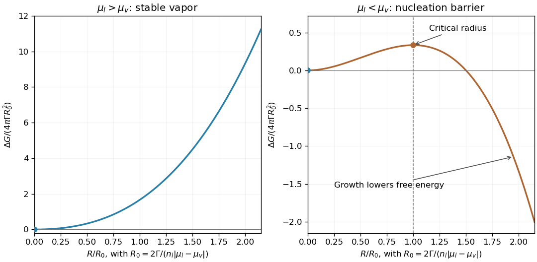
A fluctuation below $R_c$ tends to shrink because reducing its surface cost lowers thermodynamic free energy. A supercritical drop tends to grow, because its bulk free-energy gain outweighs the added surface cost. Growth continues while material supply and supersaturation allow it, eventually changing the vapor state or leading to macroscopic liquid. Curved-interface pressure and chemical thermodynamic equilibrium can also be described through the Young–Laplace equation and the Kelvin equation.

Semiconductor doping introduces electrically active impurities. In gallium arsenide, silicon has one more valence electron than gallium but one fewer than arsenic. Silicon on a gallium site can therefore supply a shallow donor electron, while silicon on an arsenic site can accept an electron and leave a mobile hole. It is an amphoteric dopant, so its net effect depends on site occupation and growth conditions.^[ref]

For isotropic parabolic bands, shift the energy origin in the given free-electron density of states to the appropriate band edge and use its effective mass:and, for valence electron states,The stated normalization includes the two spin states and assumes one effective valley. In a nondegenerate semiconductor, the conduction occupation is approximately $e^{-(E-\mu )/(k_{B}T)}$ and the probability of a valence hole is approximately $e^{(E-\mu )/(k_{B}T)}$. Substituting $x=(E-{ϵ}_c)/(k_{B}T)$ in the first integral, and the corresponding hole energy in the second, giveswhere the effective density of states values are $N_c=2[m_e{k}_{B}T/(2\pi {\hslash }^2){]}^{3/2}$ and $N_v=2[m_h{k}_{B}T/(2\pi {\hslash }^2){]}^{3/2}$. The factor $\sqrt{\pi }/2$ comes from the supplied Gaussian-weighted integral. Multiplying cancels the shared thermodynamic equilibrium chemical potential and proves the semiconductor mass-action law:For the given sample $N_D=2\times 10^{21}{\mathrm{m}}^{-3}$ and $N_A=10^{21}{\mathrm{m}}^{-3}$. With complete donor ionization and occupied acceptors, charge neutrality gives $n-p=N_D-N_A=10^{21}{\mathrm{m}}^{-3}$. At $293\mathrm{K}$ the given masses and gap giveSolving the compensated semiconductor equations, or using $n_i\ll N_D-N_A$, yieldsThe very small minority density is consistent with the wide gap and the strongly n-type balance. Also $n/N_c\simeq 2.6\times 10^{-3}\ll 1$ and $p/N_v\ll 1$, checking the nondegenerate approximation. The acceptor levels are occupied in this n-type regime; complete acceptor ionization in the compensation equation is appropriate to the model.

At low temperature dopant freeze-out reduces the conduction-electron population; a quantitative curve would require dopant binding energies and occupation factors. Once donors are ionized while intrinsic excitation is negligible, $n\simeq N_D-N_A$ gives an extrinsic plateau. At higher temperature intrinsic pairs eventually dominate, so $n\simeq p\simeq n_i(T)\propto T^{3/2}{e}^{-E_g/(2k_{B}T)}$ if the gap and masses are treated as constant. Real gap and mass changes modify that last expression.

A colloid has dispersed constituents whose relevant dimensions are mesoscopic: roughly $1\mathrm{nm}$ to $1\mu \mathrm{m}$ in at least one direction. Interfaces and Brownian motion are consequently important. The size range is a useful convention, not a sharp boundary separating all physical behaviour. A sol of fine silicon dioxide particles in water illustrates solid in liquid; an oil-in-water emulsion illustrates liquid in another immiscible liquid; and a foam illustrates gas dispersed in a liquid, with thin intervening films supplying the small structural dimension. A colloid need not be a thermodynamic equilibrium state.^[ref]

Unprotected particles attract through Van der Waals forces. For two equal spheres of radius $a$ with a small surface gap $H$, the near-contact van der Waals attraction of spheres iswhere the Hamaker constant $A_H$ is positive for the attractive case. The large number of interacting constituent molecules can give a well much deeper than $k_{B}T$, even though individual molecular attractions are weak. Brownian motion brings particles together, and a sufficiently deep attractive well makes separation unlikely. This gives particle aggregation; solid particles can remain distinct within a cluster rather than merging into one continuous solid. Emulsion droplets can additionally coalesce if the separating film ruptures.

Charge stabilization of colloids supplies a repulsive barrier. Like-charged surfaces carry compensating counterions and electric double layers; bringing the layers together costs free energy. DLVO theory combines this repulsion with Van der Waals forces. A barrier large compared with $k_{B}T$ can make aggregation slow, even when sticking would lower the final free energy. Adding salt generally shortens the Debye–Hückel screening length and can lower the barrier; surface charge regulation and specific ion interactions also matter. A negatively charged particle and a positively charged particle need not repel.

Steric stabilization instead coats each particle with adsorbed or grafted polymer chains. In a good solvent, overlap and compression of these layers raise the osmotic pressure and reduce chain entropy, opposing close contact. Electrosteric stabilization combines the two mechanisms. Dense, securely bound layers matter: incomplete adsorption can allow polymer bridging, while nonadsorbing dissolved polymers can create an attractive depletion force. Poor solvent quality can collapse a protective layer. Reducing the density mismatch slows sedimentation but does not remove the interparticle attraction, so uniform suspension and resistance to aggregation are different requirements.

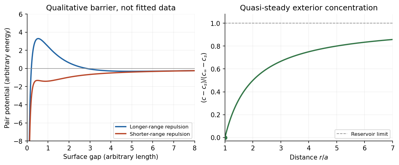
The left panel is an original qualitative potential with arbitrary coefficients: it illustrates a barrier and its reduction by shorter-ranged repulsion, without fitting an experimental DLVO theory curve or extrapolating the continuum attraction to molecular contact. The right panel plots the derived quasi-steady concentration profile in dimensionless variables.

In diffusion-controlled growth, attachment is rapid and delivery through the surrounding medium is the bottleneck. The growing surface depletes the neighboring solute, so a substantial concentration gradient develops. In reaction-controlled growth, arrival is fast compared with incorporation; many arrivals fail to attach, and the surface concentration stays near the reservoir value. The analogous distinction for particle aggregation is between near-unit sticking probability in diffusion-limited cluster aggregation and barrier-suppressed sticking in reaction-limited cluster aggregation. Here the subsequent calculation concerns accretion onto one growing particle, rather than a collision kernel for two mobile clusters.

The printed time-dependent equation is the diffusion equation, not the usual Poisson equation. For constant diffusion coefficient $D$, no bulk sources and negligible advection, Fick's laws give the number flux $\mathbf{j}=-D\nabla c$. Local conservation of mass, expressed here as conservation of the accreting constituent, then givesAn arbitrary time-independent exterior profile does not solve the full moving-boundary problem exactly. The required elementary result uses a quasi-steady approximation: diffusion establishes the exterior profile much faster than the particle radius changes. At each instantaneous radius $a$, set $\partial c/\partial t\simeq 0$. Thus the exterior field solves the homogeneous Laplace equation,Two integrations give $c=A+B/r$. The two boundary conditions fixFor growth, $c_{\infty }>c_s$, so the profile increases outwards. Its radial flux is negative, and the positive inward arrival rate isA material density is needed to turn an arrival rate into a radial velocity. Introduce the constant constituent number density $c_p$ inside the particle, using the same units as $c_s,c_{\infty }$. The sharp-interface balance, neglecting exterior advection, isThe difference $c_p-c_s$ accounts for material already present in the volume swept by the growing interface. In the usual dilute-feed approximation $c_s\ll c_p$, it can be replaced by $c_p$. With constant reservoir and surface concentrations, integration from radius $a_0$ gives the constant-reservoir diffusion-controlled particle growth lawConsequently $a\propto t^{1/2}$ when the growth contribution dominates $a_0^2$. For a finite seed at the literal limit $t\to 0$, the increment $a-a_0$ is instead initially proportional to $t$. Here “early time” means before appreciable reservoir depletion or interactions with other particles, while already beyond the rapid initial establishment of the diffusion field. Indeed, the ratio of diffusion-adjustment time $a^2/D$ to radial-growth time $a/\dot{a}$ is $(c_{\infty }-c_s)/(c_p-c_s)$; small supersaturation relative to the particle density makes the quasi-steady approximation self-consistent. No initial concentration field was specified, so an exact transient solution is not uniquely determined.

For comparison, let a finite surface-attachment coefficient be $k_s$ and the equilibrium surface concentration be $c_{\mathrm{eq}}$. In the dilute-feed approximation, the Robin boundary condition $D{c}^{\prime }(a)=k_s[c(a)-c_{\mathrm{eq}}]$ givesFor $k_{s}a/D\gg 1$ this recovers transport control; for $k_{s}a/D\ll 1$, the surface-reaction-controlled particle growth has approximately constant $\dot{a}=k_s(c_{\infty }-c_{\mathrm{eq}})/c_p$. Thus reaction control gives $a-a_0\propto t$, in contrast to the diffusion-controlled square-radius law. No numerical $c_p$ or $k_s$ is supplied or needed for these scaling results.