Aerospace engineering concerns aircraft and spacecraft, linking aerodynamics, structures, propulsion, control and thermal design. Aircraft operate through forces exchanged with the atmosphere; spacecraft also require orbital dynamics and operation in vacuum. A low-mass structure can reduce propulsion requirements but may be more flexible, affecting control and vibration. Coupling these subsystems makes performance a system-level property: improving one component's isolated efficiency does not necessarily improve the complete vehicle.
The area rule is an aerodynamic design principle relating transonic wave drag to the longitudinal distribution of the total cross-sectional area of an aircraft, including its fuselage and aircraft wings. A wing-body combination can create a rapid area increase even when each part appears streamlined in isolation. Redistributing the fuselage area near the wing can smooth the combined distribution. This does not say that any reduction in frontal area guarantees lower total drag.[ref]
Richard T. Whitcomb by NASA. Area-rule account, combined cross-sectional-area distribution and wing-body model test
An original geometric model makes the redistribution explicit. Let increase along the fuselage, and let and denote body and added-wing areas, counting their overlap only once. Over a stipulated interval of length , takeIf the desired combined distribution on that interval is , the bookkeeping choice gives . For , and , the body's area is at the midpoint. Relative to a constant-area body, the removed volume isThis invented example exposes a design tradeoff: smoothing an area distribution can consume internal volume. It is not a calculation of wave drag, and the rest of the vehicle still needs smooth transitions.
Richard T. Whitcomb's motivating test used a specially built wing-body model in a wind tunnel, before applying the shape change to a fighter configuration. Comparing measured drag through the transonic range tests the proposed area-distribution effect; appearance alone does not. Viscous stress, lift-induced drag, loading and off-design conditions still matter to the complete aircraft.[ref]
The National Advisory Committee for Aeronautics was the United States' aeronautical research organization established in 1915. Its laboratories and personnel formed the core of the National Aeronautics and Space Administration in 1958. Its technical legacy includes wind tunnels, systematic NACA airfoil families and published measurements that let designers compare aircraft wings.[ref]
The National Advisory Committee for Aeronautics by NASA. Agency history,1915–1958
A particularly useful research strategy was to change geometry systematically while keeping test conditions comparable. Eastman N. Jacobs, Kenneth E. Ward and Robert M. Pinkerton varied airfoil thickness-to-chord ratio and airfoil camber in their related-section experiments, rather than testing only unrelated existing designs. The measurements connected an explicitly specified shape with lift coefficient, drag and pitching moment.[ref]
The Characteristics of 78 Related Airfoil Sections from Tests in the Variable-Density Wind Tunnel by Eastman N. Jacobs and others. Summary and Introduction, systematic shape variables
An original similarity calculation illustrates why the apparatus mattered. A small model with airfoil chord in air of density , dynamic viscosity and speed has Reynolds numberA five-times-larger chord at the same conditions has . A variable-density wind tunnel can instead raise the model's air density fivefold to match that Reynolds number, approximately holding dynamic viscosity fixed. Matching it alone does not also establish matching Mach number, surface condition or wind-tunnel turbulence intensity.
The enduring contribution is a reusable experimental comparison: specify shape, operating conditions and how forces were measured, then publish results that can be checked against another experiment or computational fluid dynamics calculation.
An aircraft is a vehicle capable of flight through the atmosphere. Its support can involve aerodynamic lift or buoyancy. A fixed-wing aircraft obtains aerodynamic lift from its aircraft wings as it moves relative to the surrounding air. An engine can supply thrust, but propulsion and the aerodynamic support of gravitational weight are distinct functions.[ref]
For straight, level flight at constant velocity, neglect vertical thrust and align the remaining thrust with the flight direction. The force balance isHere is lift, is drag, is thrust and is gravitational weight. For a stipulated vehicle with and lift-to-drag ratio , this requires and . At an air-relative speed of , is the useful propulsive mechanical power; an engine's input power can be larger because of losses.
An unpowered glider can instead maintain a steady descending velocity. If its glide angle below the horizontal is , resolving gravitational weight perpendicular and parallel to the flight path givesConsequently an assumed constant corresponds to and 12 units of horizontal travel per unit of height lost in still air.[ref] The loss of gravitational potential energy supplies the work against drag; the kinetic energy need not be falling during that steady descent.
These balances concern translation of the vehicle. Maintaining its orientation also requires a balance of torques about its centre of mass. An aircraft can satisfy an instantaneous vertical force balance while still having an unwanted pitching moment.
The aircraft yaw axis is the body-fixed axis about which the nose rotates from side to side. In a right-handed body coordinate system with forward and toward the right wing, it is the axis directed downward through the centre of mass. It completes the orthogonal set with the aircraft roll axis and aircraft pitch axis. The rudder can generate a side force aft of the centre of mass, producing a yawing torque.[ref]
Aircraft Rotations by NASA Glenn Research Center. Yaw axis and final control-surface discussion
For a force acting at displacement from the reference point, the yaw component of isIn an original example, a rightward tail force at gives . With positive yaw defined nose-right, this force turns the nose left. If the axis is a principal axis with moment of inertia and the initial motion is pure yaw, the instantaneous angular acceleration is . A tail's displacement matters as well as the force magnitude.
The aircraft yaw rate is a component of body angular velocity; it is not always the rate of change of aircraft heading. A banked vehicle projects its rotation onto several body axes, and its ground track also depends on wind. General coupled motion uses Euler's equations, rather than three independent scalar torque laws. Measuring a heading change alone therefore cannot establish the applied yawing moment.
The aircraft roll axis is the longitudinal body axis through the centre of mass, conventionally directed toward the nose. Positive rotation around that forward axis lowers the right wing in the right-handed system with right and down. An aileron changes the aerodynamic loading of a wing; unequal loads on opposite sides can generate a rolling torque.[ref]
The roll component of isAn original pure-couple example places an upward incremental force of at and a downward incremental force of the same magnitude at . With both application points at , their total incremental force vanishes butThe negative sign means right-wing-up rotation. For an initially pure roll about a principal axis with moment of inertia , the instantaneous angular acceleration is . This is a stipulated force couple, not an aileron-performance prediction.
The aircraft roll rate describes rotation, while bank angle describes attitude relative to a local horizontal reference. A vehicle held at a constant bank angle can have zero change of that angle while its flight direction turns. Conversely, a rolling aircraft need not already have the steady centripetal force required by the fixed-wing aircraft turning model. Attitude, angular velocity and trajectory are separate measured quantities.
The aircraft pitch axis is the transverse body axis about which the nose rotates upward or downward. In the convention used by NASA Glenn Research Center, it passes through the centre of mass and points toward the right wing tip; the aircraft roll axis points toward the nose and the aircraft yaw axis toward the underside. These are body-fixed directions, so their orientation relative to the ground changes with the aircraft.[ref]
Aircraft Rotations by NASA Glenn Research Center. Pitch axis, Roll axis and Yaw axis
Choose right-handed body coordinates forward, right and down. A force acting at displacement from the centre of mass produces torque . Its pitching moment isFor an original tail-load example, and give . The downward tail load lifts the nose in this convention. If the aircraft pitch axis is a principal axis, the motion is initially pure pitch and the corresponding moment of inertia is , then the instantaneous angular acceleration is . Coupled three-axis rotation requires the full Euler's equations.
The axis is a geometrical reference, not necessarily a physical hinge. Changing a control-surface load changes both forces and torques; a zero net translational force does not establish zero pitching moment. A balance measurement therefore needs the reference point and sign convention alongside its reported moment.[ref]
Groundspeed is the magnitude of an aircraft's horizontal velocity relative to the ground. It determines travel time along a ground track, whereas aerodynamic lift and drag depend on motion relative to the air. Let and be the horizontal ground-relative and air-relative velocity vectors, and let be the horizontal wind velocity:For climbing or descending flight this horizontal convention distinguishes groundspeed from the magnitude of the full three-dimensional ground-relative velocity.[ref]
In an original horizontal-flight example, an airspeed of directed due north and a wind blowing east at give in east/north coordinates. Thus , with the track about east of north. Adding scalar speeds would wrongly give .
To keep a due-north track in the same wind, the aircraft must instead supply an air-relative westward component of . At the same airspeed, its northward component becomes , so the on-track groundspeed is smaller than the airspeed. The required wind correction angle is west of north. Heading and track are distinct directions.
Timed positions from a ground-based tracker estimate groundspeed, not airspeed. Inferring the latter also needs the wind velocity. Conversely, a Pitot-static tube does not measure travel over the ground. The same distinction explains why a headwind changes the ground range of a steady glider without changing its air-relative glide angle.
The wind correction angle is the difference between the aircraft heading and the desired ground track needed to compensate for a crosswind. A heading points the vehicle; a track describes horizontal travel over the ground. In the horizontal model here, the air-relative velocity is aligned with the heading. Wind-direction statements below specify where the air moves, not the meteorological direction it comes from.[ref]
Relative Velocity by NASA Glenn Research Center. Ground Reference and Wind Speed, reference-frame relation
Let be true airspeed, let be wind along the desired track, and let be wind to its right. Define a positive correction as heading right of the track. Cancelling cross-track velocity and projecting along the track givesFor the branch with a nonnegative along-track air-relative component,The condition permits crosswind cancellation, but forward progress also requires .
In an original example, take , wind rightward and opposite the intended track. Then and . A constant-condition ground leg takes about . With the same headwind, a rightward component of can still be cancelled, but : the resulting track-line motion is backward.
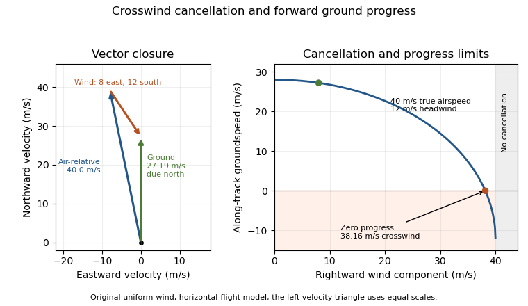
An original wind triangle and forward-progress limit at fixed true airspeed. Cancelling crosswind alone does not guarantee progress against a headwind.
Details. The calculation assumes a uniform horizontal wind and a steady true airspeed. Ground-position measurements can test the resulting groundspeed; they cannot determine the correction from air-relative speed alone without wind information. Wind variation and a difference between heading and air-relative velocity require a fuller vector model.
Airspeed describes an aircraft's motion relative to the surrounding air. When the kinematic magnitude is intended, it is the true airspeed,It differs from groundspeed whenever wind changes the relative motion. A ground-station velocity alone cannot establish the aerodynamic airspeed.[ref]
An airspeed instrument normally infers motion from pressure. At low Mach number, for an aligned Pitot-static tube in the regime of the Bernoulli equation,Here is stagnation pressure, is static pressure and is air mass density. For a stipulated difference of , gives ; the same difference at gives . The instrument senses a pressure difference, so interpreting its reading requires a density model and an instrument calibration.[ref]
Pitot – Static Tube – Speedometer by NASA Glenn Research Center. Pressure connections, Solve for Velocity and Limitations
Indicated airspeed is the displayed reading before instrument and installation corrections. Calibrated airspeed includes those corrections. True airspeed expresses actual motion through the air, rather than simply relabeling either reading. The FAA distinguishes these quantities in its instrument chapter.[ref]
The square-root calculation above assumes an appropriate low-speed stopping relation. At appreciable Mach number, compressibility changes that relation; a blocked passage or displaced static pressure source introduces a different measurement problem. Report which airspeed convention and corrections accompany a performance curve. Comparing speeds without that information can confound a change of air mass density with a change in the aircraft's loading. Functioning ports and known corrections are part of the inference, not extra measurements of groundspeed.
Calibrated airspeed is indicated airspeed corrected for instrument and installation errors. It remains a pressure-based speed convention; correcting the indicator does not by itself convert the reading into true airspeed. The FAA uses an airspeed-calibration chart to distinguish the indicated and corrected values.[ref]
Represent a specified correction chart byThe correction can depend on the operating condition. In an original invented chart, suppose indicated and correspond to calibrated and . Linear interpolation over this stipulated interval givesso an indication of maps to . Neither a constant correction nor a universal percentage reproduces both chart endpoints. Extrapolation outside the measured interval is an additional assumption.
At low Mach number, corrected pressure difference is approximately , with the standard reference air mass density. The example's corrected pressure estimate is times the estimate obtained by treating the indication as calibrated. The corresponding correction to an inferred aerodynamic force at fixed coefficient and area is therefore not merely the speed correction.
Instrument testing checks the mapping from applied pressures to the reading. Installed-system work also addresses static-pressure position error: a port can sample a local pressure different from the intended free-stream static pressure. The correction must accompany its configuration and reference conditions. To obtain true airspeed, account for ambient conditions as well. At appreciable Mach number, compressibility also separates calibrated and equivalent airspeed; the low-speed square-root density conversion must not be silently extended to that regime.
Indicated airspeed is the airspeed read directly from an indicator before correcting its instrument and installation errors. It is a displayed measurement, not automatically the aircraft's true airspeed or groundspeed. A conventional Pitot-static tube supplies total and static pressure through separate connections; the indicator converts their difference into a speed reading.[ref]
A simple low-Mach number instrument model uses a standard reference mass density and the sensed difference :This formula describes the stipulated ideal scale; real instrument errors need separate characterization. In particular, using does not assert that local air has that mass density.
For an original error example, let the actual total-minus-static difference be , but suppose the static connection reads too high while the total-pressure connection is correct. Then . With , the model shows instead of . A positive error in one input has become a negative error in the difference. At lower pressure differences, the same offset has a larger fractional effect on the indicated speed.
A pressure-bench check can apply known differences to the instrument and test its zero and scale. It cannot alone characterize static-pressure position error caused by the ports' location on the flying aircraft. Calibrated airspeed accounts for the established instrument and installation corrections. A blocked port is another failure mode: treating every discrepancy as a correctable constant offset would conceal a changing or trapped pressure signal. The FAA specifically identifies obstruction and instrument deterioration as causes of incorrect indications.[ref]
Glider Flying Handbook by Federal Aviation Administration. Chapter 4, printed p. 4-5, Calibrated Airspeed and pitot obstruction
True airspeed is the magnitude of an aircraft's velocity relative to the surrounding air,It determines the relative motion used in aerodynamic models, while groundspeed concerns horizontal travel over the ground. Indicated airspeed and calibrated airspeed describe stages in a pressure-instrument reduction, rather than another reference frame.[ref]
For an aligned low-Mach number pressure measurement in the regime of the Bernoulli equation,An equivalent airspeed uses the same dynamic pressure with a standard reference mass density, . HenceOnly where the low-speed pressure relations justify may calibrated speed be substituted in this last expression without a separate compressibility correction.
For an original low-speed example, use , and ambient . The corrected difference is approximately , giving . At a fixed pressure difference, halving ambient mass density increases the inferred true airspeed by , rather than doubling it. This follows from the square-root dependence, not a wind correction.
Obtaining the ambient mass density can require independent static pressure and thermodynamic temperature measurements, with a suitable equation of state. For fixed , a small relative density error changes the inferred speed by approximately . Wind information is needed separately to predict the ground track. A single ground-travel speed cannot supply all of these quantities. The pressure inference also depends on clear passages and valid stopping-flow assumptions.[ref]
Pitot – Static Tube – Speedometer by NASA Glenn Research Center. Solve for Velocity and Limitations
A fuselage is the main body of a conventional aircraft, accommodating payload or equipment and connecting major assemblies such as the aircraft wings. It is part of the load-carrying structure as well as the aerodynamic shape. Not every aircraft has a separate conventional fuselage, and not every fuselage is pressurized.[ref]
Fuselage by NASA Glenn Research Center. Fuselage and Weight, accommodation, component connections and applied torques
The structural role is more than enclosing a volume. Forces from attached assemblies and distributed gravitational weight must be transmitted through the body, producing bending, shear and axial loading. A pressurized body also carries loads from the pressure difference between its interior and the atmosphere. These are different loading mechanisms, even if they act on the same shell.
An original ideal model illustrates the pressure contribution. Approximate a closed cylindrical section as a thin-walled pressure vessel of radius , wall thickness and internal excess pressure . Force balance across a longitudinal cut of length gives . Balance of an end cap gives . ThusThe first is hoop stress and the second axial stress. For , and , they are and . This stipulated membrane model excludes cutouts, joints, stiffeners and aerodynamic bending; it is not a complete fuselage stress analysis.
Shape also affects the combined flow around the body and wings. Richard T. Whitcomb's area rule work examined the longitudinal area distribution of the entire combination, rather than judging the wing and fuselage as isolated streamlined parts. That connection explains why structural packaging and aerodynamic design cannot always be optimized independently.
A fixed-wing aircraft obtains most of its aerodynamic support from aircraft wings that do not continuously rotate around a shaft to generate lift. The word fixed distinguishes the lifting arrangement; it does not require every surface to be immovable or perfectly rigid. Both powered airplanes and an unpowered glider can use fixed wings.
Thrust and aerodynamic support are distinct. Relative motion through air produces lift and drag; an engine can supply the thrust needed to balance drag in steady level flight. The components must be resolved as vectors, since their directions change with the motion and attitude.[ref]
For an original ideal turning model, suppose a point-mass aircraft maintains horizontal circular flight at constant airspeed , with negligible vertical thrust and no net vertical acceleration. If its lift vector is inclined through a bank angle , thenThe horizontal component supplies centripetal acceleration. Eliminating gives and . With , and , the radius is about and the required lift is about . The wing remains fixed to the body while its force direction changes in space.
This is a Newtonian force model, not a prediction that an arbitrary airplane can produce the required lift. The attainable lift coefficient, wing loading, propulsion and aerodynamic moments determine whether a particular steady condition can exist. In a steady unpowered descent, the balances instead lead to the glide angle relation.
The bank angle measures an aircraft's lateral tilt relative to a local horizontal reference. In the ideal fixed-wing aircraft turning model, the lift vector tilts with the vehicle. For more general motion, vehicle attitude, flight-path direction and aerodynamic force direction must be distinguished; a banked vehicle need not follow a level circle.[ref]
Aircraft Rotations by NASA Glenn Research Center. Roll axis, wing-tip motion and attitude-control discussion
For steady horizontal circular motion with negligible vertical thrust and lift tilted by , the force balance developed in fixed-wing aircraft gives the aerodynamic load factorAt , the required lift is twice the gravitational weight. If the maximum usable lift coefficient is held fixed, implies the model's limiting airspeed scales asA stipulated wings-level limit of therefore becomes at this loading. This is a comparison at fixed configuration and air mass density, not a claim that a particular aircraft can sustain the required condition. Aerodynamic stall and structural limits constrain the accessible turn.
A banked glider also needs a different loading balance from the shallow straight-glide model used to define minimum sink speed. Increasing bank angle cannot be analyzed merely by rotating a drawing of its still-air trajectory. Measured performance must specify the turn condition as well as airspeed; the FAA's performance discussion illustrates how bank and loading affect glider operation.[ref]
The aerodynamic load factor compares lift with gravitational weight. The stated convention takes along the chosen positive lift direction, so is a signed force ratio, not simply the magnitude of total acceleration divided by . A steady level condition can have with zero inertial acceleration.[ref]
Introduction to Aircraft Performance and Static Stability by Earll Murman. PDF pp. 14–15, Horizontal Turn and Pull Up/Pull Over/Vertical
A focused example is a wings-level pull-up at the bottom of a vertical curved path. Neglect other vertical forces and take upward normal acceleration as positive. The force balance givesFor stipulated true airspeed , curvature radius and , the upward centripetal acceleration is and . With , lift is , while the net upward force is . Neither is the other.
In the steady horizontal-turn model, the condition instead is ; bank angle derives that balance. It does not apply unchanged to the vertical pull-up. At fixed air mass density, wing area and usable maximum lift coefficient, the relation gives limiting speed proportional to for positive . For this example, the factor is about relative to the corresponding one-load condition.
A force balance measures aerodynamic load; a trajectory measurement estimates inertial acceleration. Comparing them requires the gravitational weight term and correct directions. A reported load factor also needs its force-axis convention: thrust, side forces and coupled motion can matter to what an instrument actually records. The definition alone establishes neither structural capability nor available lift before aerodynamic stall.
The glide angle is the inclination of a descending flight path below the horizontal. A positive will denote descent here. For aerodynamic reasoning it is important to specify motion relative to the air: a steady wind can change the ground track without changing the air-relative glide angle at the same operating condition.
For a steady unpowered descent, resolve gravitational weight perpendicular and parallel to the air-relative velocity. With lift normal to that velocity and drag opposing it,The still-air horizontal distance per unit height lost is therefore . NASA's description connects this geometry with a historical observation: the Wright brothers flew parallel to a dune slope, letting the slope provide an estimate of the flight-path angle.[ref]
For an original constant-velocity model, set and airspeed . Then , horizontal air-relative speed is , and downward speed is . In still air, a stipulated height loss corresponds to horizontally.
If a constant horizontal wind component is positive along the direction of travel, the ground-frame horizontal speed is . With no vertical wind and ,A headwind makes that ratio about ; a tailwind of the same magnitude gives . All three cases retain the same air-relative angle and sink rate. Their groundspeeds and ground-frame path angles differ.
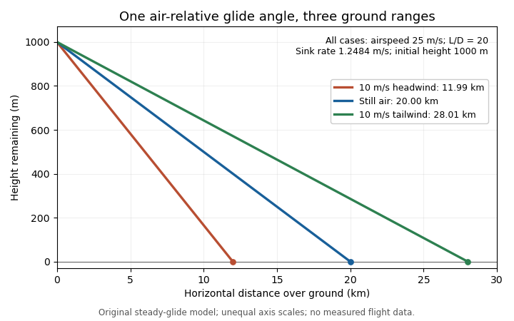
The same air-relative glide condition gives different ground ranges in a stipulated constant headwind, still air and tailwind. Original model; unequal plotting scales mean displayed line angles are not the physical glide angles.
Details. This distinction separates a measured ground trajectory from an aerodynamic lift-to-drag ratio. Estimating the latter from height and horizontal travel requires accounting for air motion and identifying the steady portion of the trajectory.
A glider is an aircraft designed for sustained flight without continuous engine thrust. Its aircraft wings obtain aerodynamic lift from motion relative to the air. It can descend steadily while its speed remains constant: loss of gravitational potential energy, rather than a continuous reduction of kinetic energy, can supply the work against drag.[ref]
Four Forces on an Airplane by NASA Glenn Research Center. Gliders and the distinction between propulsion and aerodynamic support
In still air and a steady unpowered glide, the mechanical power balance iswhere is airspeed and is downward speed. This follows from and in glide angle. Motion of the surrounding air changes the ground-relative energy account; rising air can offset a glider's descent relative to that air.
Two performance objectives should be distinguished. The minimum sink speed minimizes the downward rate, while the best glide speed maximizes horizontal distance per unit height lost in still air. They need not be the same speed.
For an original comparison, stipulate two steady operating points: with , and with . Their horizontal-distance ratios areAmong these two stipulated points, the slower one stays aloft longer for a given height loss, but the faster one covers more horizontal distance. From , the corresponding times are about and . These invented points illustrate the competing objectives; they are not a measured performance curve.
A simple motivating experiment tracks a small unpowered model's position and height through a nearly steady portion of flight, then compares the vertical and horizontal motion. NASA identifies paper and lightweight model gliders as accessible examples.[ref] Repeating with controlled geometry and launch conditions distinguishes the resulting motion from a claim based solely on a large wing aspect ratio.
A glider sink polar relates a glider's steady downward speed relative to the air to its true airspeed, for specified loading, configuration and atmospheric conditions. Write it as with downward motion positive. Some plots instead put descent below the horizontal axis; the sign convention must accompany the curve. The minimum sink speed and best glide speed select different points on this same performance relation.[ref]
The curve is a measurement or model of performance, rather than a drawing of the flight path. At steady speed, its horizontal air-relative component is . Thus time per height lost is , while horizontal distance per height lost is . The best glide speed article derives the tangent construction and an original parabolic drag polar example; those results need not be recomputed to interpret a measured polar.
A useful extension is glider ballast scaling. Suppose the gravitational weight changes from to at unchanged air mass density and geometry, and suppose the same lift coefficient and drag coefficient remain applicable. At corresponding steady glide conditions, the lift-to-drag ratio and glide angle are unchanged. Since ,For an original stipulated point and , increasing gravitational weight by gives and . The corresponding distance-to-height ratio is unchanged, but the same height is lost sooner. This scaling assumes the aerodynamic coefficients transfer; changes of Reynolds number, surface condition or trim can invalidate it. The FAA illustrates the loading-dependent displacement of glider polars.[ref]
To measure a polar, record steady true airspeed and height change at several operating points while documenting configuration and loading. Ground-relative descent includes vertical motion of the air: with upward air velocity , . For example, an air-relative sink of in air rising at appears as ground-relative descent. Repetition can reveal variability, but one trajectory cannot separate these two contributions without additional information. A measured groundspeed is likewise not automatically the horizontal component of the air-relative polar.
The best glide speed is the airspeed giving the greatest horizontal distance per unit height lost in a specified steady glide condition. In still air this is the speed for maximum lift-to-drag ratio. It differs from the minimum sink speed, whose objective is longest time aloft for a given height loss.[ref]
Write a glider sink polar as downward rate . The horizontal air-relative speed is , so the exact still-air range per unit height is . For a shallow glide angle, and maximizing range is approximately minimizing . At an interior optimum,Geometrically, a line from the origin is tangent to the positive-downward-rate polar. This is not the horizontal tangent defining minimum sink speed.
For an original calculation, take a parabolic drag polar and approximate . At fixed air mass density , wing area and gravitational weight ,Minimizing givesStipulate , , , and . Then , in the corresponding SI units, , and the model gives . Its shallow-glide range ratio is . These parameters are invented; an attainable lift coefficient and a valid drag polar are prerequisites, not consequences of the optimization.
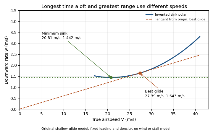
Minimum sink and best glide are different optima of an original shallow-glide polar. Positive vertical values denote downward speed; the curve is an invented model, not measured aircraft performance.
Details. Wind changes the ground-range objective to for an along-track wind component and no vertical air motion. Therefore the still-air optimum need not maximize ground distance. The FAA constructs the corresponding shifted tangents on its performance polars.[ref]
Glider Flying Handbook by Federal Aviation Administration. Chapter 5, printed pp. 5-10–5-11, wind and sinking-air polar constructions
A controlled performance measurement records steady airspeed and height loss at several speeds; wind, vertical air motion and changes of loading must be distinguished from the polar itself.The minimum sink speed is the airspeed at which a glider has its smallest steady downward speed relative to the air, for a specified configuration, loading and flight condition. It maximizes time aloft from a given height in still air. It does not generally maximize horizontal range, which defines best glide speed.[ref]
For a differentiable glider sink polar , an interior minimum satisfies , with a positive second derivative sufficient for a strict local minimum. For the original shallow-glide model developed in best glide speed,With , this givesIndeed for . The speed ratio is about , within this stipulated parabolic drag polar approximation. A real polar need not follow that numerical ratio, especially near aerodynamic stall.
Using the same original , and gives and . From a stipulated height, the model's times are about at minimum sink and at best glide. Yet the approximate range ratios are and , respectively. The slower optimum buys time rather than maximum distance.
A horizontal wind changes range without changing air-relative sink at a fixed condition. Vertical air motion changes ground-relative height loss as well: descending at through air rising at gives ground-relative descent . Observing constant height therefore does not establish zero air-relative sink. A bank angle also changes the required lift and hence the appropriate polar; the straight-glide optimum cannot simply be reused for a tight turn.
An aircraft wing is an aerodynamic lifting structure of an aircraft. Its three-dimensional shape combines airfoil sections with a spanwise arrangement described by the wing planform. The airfoil specifies a local profile; the wing planform specifies the shape seen from above. Wingspan, wing area, wing taper ratio and wing sweep describe different aspects of that geometry.[ref]
Wing Geometry by NASA Glenn Research Center. Top View and Airfoil Geometry: span, planform and sectional shape
The surrounding fluid flow exerts pressure and viscous stress on the wing's surface. Integrating these surface forces gives a resultant whose component perpendicular to the incoming flow is lift and whose parallel component is drag. A useful whole-wing relation iswhere is air density, is flight speed relative to the air, is wing area and is lift coefficient. The lift coefficient packages the effects of shape and operating conditions, including angle of attack; it is not determined by wing area alone.
For a stipulated example, , , and give dynamic pressure and lift . Halving the speed at unchanged lift coefficient reduces lift to one quarter. Maintaining the original lift would require , which the actual wing might be unable to achieve before aerodynamic stall.
A wind tunnel makes the shape–force connection measurable: hold a model at controlled angle of attack, measure its lift and drag with a balance, and vary the model or flow conditions. Such measurements distinguish a geometrical description from an aerodynamic prediction. Two wings with equal wingspan and wing area can still have different lift coefficients, drag and stall behavior.
A winglet is a small wing-tip lifting surface, often inclined upward out of the main wing planform. By changing the three-dimensional loading and flow near the tip, it can reduce lift-induced drag. Its winglet cant angle, shape and attachment must be considered with the entire aircraft wing; it is not a universal bolt-on reduction in total drag.[ref]
A Design Approach and Selected Wind-Tunnel Results at High Subsonic Speeds for Wing-Tip Mounted Winglets by Richard T. Whitcomb. NTRS author abstract, geometry and measured aerodynamic effects
Richard T. Whitcomb's 1976 report compared measured forces, moments and loads on a representative transport wing with and without wing-tip devices. A particularly useful comparison was a tip extension giving approximately the same increase of bending moment at the wing–fuselage junction as the winglets. That comparison asks how much aerodynamic benefit is obtained for a similar structural penalty, rather than comparing only nominal span.[ref]
A Design Approach and Selected Wind-Tunnel Results at High Subsonic Speeds for Wing-Tip Mounted Winglets by Richard T. Whitcomb. Abstract, matched bending-moment increment for tip-extension comparison
An original coefficient budget illustrates why component and total benefits differ. Keep the same reference wing area, dynamic pressure and lift coefficient. Suppose initiallywhere the second term is the lift-induced drag contribution. If a proposed modification reduces that term by but adds to other drag coefficient contributions, thenThe total reduction is about , not . This is an invented budget, not a prediction or a measured winglet efficiency. Increased loading, additional wetted area and an off-design operating point can change the result.
A convincing wind tunnel comparison measures total drag at matched lift, records moments and loading, and documents how the mounting correction and reference area are handled. A photograph of a weaker-looking wingtip vortex is not a measurement of total drag. Conversely, reducing lift-induced drag does not require all three-dimensional trailing vorticity to disappear.
The winglet cant angle specifies the inclination of a winglet away from a stated reference direction. Here means an upright winglet, with positive tilting outward from vertical in the transverse plane. A convention measured upward from the main wing plane would instead give for this ideal geometry. A quoted angle therefore needs its reference plane. Winglet toe angle concerns a different orientation, involving the chord and incoming flow.
For a straight unswept winglet of length , the purely geometric projections areIf symmetric winglets attach at the tips of a main wingspan , their outer-tip projected separation is . With stipulated , and , the vertical height is , each tip moves outward , and the total projected separation is about . None of these projections alone supplies a new span efficiency factor or a prediction of lift-induced drag.
Cant also changes how loads act on the supporting wing. In a right-handed frame with outward, upward and completing the triad, the rolling-moment contribution of an applied force is . For a stipulated vertical force applied at the outer tip, the moment about the vehicle centreline is when the winglet is upright and about at the stated outward cant. This isolates the changed moment arm; an actual aerodynamic load need not stay vertical or keep the same magnitude when cant changes.
Richard T. Whitcomb's primary design discussion explicitly balances lift-induced drag, skin friction and wing bending moments, and discusses outward cant separately from incidence and twist. It also identifies interference at the upper-winglet root as part of the design problem.[ref]
A Design Approach and Selected Wind-Tunnel Results at High Subsonic Speeds for Wing-Tip Mounted Winglets by Richard T. Whitcomb. Printed pp. 7–8, Incidence and twist and Cant or dihedral
A controlled wind tunnel comparison must therefore record forces and moments at matched conditions, rather than infer an optimum cant solely from the projected span.A swept wing has a specified spanwise reference line inclined relative to the direction perpendicular to the aircraft's longitudinal axis. Aft sweep places the outboard part farther rearward; forward sweep places it farther forward. The leading-edge sweep angle and quarter-chord sweep angle can differ, so a sweep value needs a named reference line.[ref]
Applied Computational Aerodynamics by W. H. Mason. Appendix A, pp. A-27–A-29, planform coordinates and sweep relations
A useful geometric construction shifts each spanwise strip of a wing planform fore or aft while retaining its local airfoil chord. If both edges receive the same shift, their separation and hence the integrated wing area remain unchanged. For an original constant-chord example with wingspan and , define . The tip leading edge is aft of the root, while and are unchanged by the strip shift.
Preserving these geometric scalars does not preserve the three-dimensional flow. At high Mach number, the normal Mach number for a swept leading edge helps organize a simplified comparison of the component perpendicular to that edge. Finite-span flow, thickness and interference with the fuselage remain relevant.
The primary 1947 experiment by Richard T. Whitcomb used a different geometric change: it rotated the two wing semispans to obtain zero, forward and backward sweep, then obtained loading and drag information from pressure measurements and wake surveys. The shock-associated changes did not shift by exactly a universal cosine factor.[ref]
Thus an experimental sweep comparison should identify what changed besides the angle: rotation of an existing wing, a stripwise shear of a planform, and a newly designed swept wing need not retain the same projected area or section arrangement.
Wing loading is the gravitational weight of an aircraft divided by its reference wing area:It is a whole-aircraft loading measure. In SI its units are , not . The latter units describe mass per wing area, , and require multiplication by gravitational acceleration to obtain .
For an original unit check, , and give but . Although this has the units of pressure, it is not the local pressure distribution on the wing surface.
In straight level flight with negligible vertical thrust, lift balances gravitational weight.[ref] Combining this with the definition of the whole-wing lift coefficient givesAt fixed air mass density and required coefficient, airspeed therefore scales as the square root of wing loading. For stipulated , and , the result is . Doubling only the loading gives , a factor of .
If a model assumes a maximum attainable , the same equation gives a corresponding minimum speed for that straight-level condition. It is not a universal speed for every attitude or configuration: a turning condition can require , and a changed airfoil, surface condition or Reynolds number can change the attainable coefficient.
A geometric and weighing check determines , the relevant loading state and projected wing area. Those measurements establish ; a separate aerodynamic experiment is needed to establish the applicable lift coefficient. Equal wing loading does not establish equal lift-to-drag ratio or identical aerodynamic stall behavior.
The wing aspect ratio is the dimensionless measurewhere is wingspan and is projected wing area. For a rectangular wing planform, and therefore , where is airfoil chord. For other wing planforms, dividing the span by a chosen root chord need not give the wing aspect ratio.[ref]
Its aerodynamic importance comes from lift-induced drag. The wingtip vortices of a finite aircraft wing change the local flow direction; maintaining lift then entails an additional rearward force. A standard model writesHere is a span efficiency factor, is dynamic pressure and is lift coefficient. The model compares a specified spanwise loading in a regime where this finite-wing approximation is appropriate; need not stay unchanged when the design changes.[ref]
Induced Drag Coefficient by NASA Glenn Research Center. Induced Drag Coefficient, aspect ratio and efficiency
For an original example, take , , and . Both wings then supply . Spans of 8 and 12 metres give and , respectively, and lift-induced drag approximately and . Under those stipulated conditions, increasing span by 50% reduces that drag component by , about 55.6%.
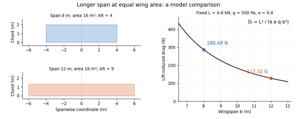
Equal-area wings with different span, and the inverse-square induced-drag comparison at fixed lift, dynamic pressure and span efficiency. Original model calculation.
Details. The boxed expression also exposes a common comparison error. At fixed , , and , changing only the reference wing area changes both wing aspect ratio and lift coefficient; their effects cancel in this model's dimensional lift-induced drag. A larger numerical is therefore not, by itself, a promise of smaller total drag. Structural loads, wing loading, surface losses and aerodynamic stall impose further design constraints.
The wingspan of an aircraft wing is its lateral tip-to-tip extent. For a symmetric wing planform, a spanwise coordinate runs from at one tip to at the other; the semispan is . This geometrical distance differs from the local fore-and-aft airfoil chord.[ref]
Wing Geometry by NASA Glenn Research Center. Top View: tip-to-tip span and chord directions
Together with wing area , the wingspan defines the dimensionless wing aspect ratio,For a rectangular wing planform of constant airfoil chord , , giving . For example, a wing with and has . A second wing with the same wing area but has . Equal wing area therefore does not imply equal lateral slenderness.
There is also a simple structural reason why the span matters. Suppose a symmetric wing supplies total upward lift , distributed uniformly along its span. On one half-wing the resultant load is and acts from the center. The corresponding bending moment at the center isFor and this gives . This is an idealized aerodynamic loading calculation: the actual load distribution, structural supports and component masses modify the wing's bending moment. It nevertheless shows why increasing wingspan affects the structure as well as the wing aspect ratio.
A wing planform is the two-dimensional outline of an aircraft wing viewed from above. It is bounded by the projected leading edge, trailing edge and wing tips. A rectangular, tapered or swept wing planform can be combined with many different airfoil profiles; the outline alone does not specify the wing's thickness or airfoil camber.[ref]
Let point aft and run along the wingspan. Describe the two edges by and . Their separation is the projected local airfoil chord,The second equation computes wing area. The first retains information lost by that single area value: where the chord lies along the fore-and-aft direction.
For an original comparison, a rectangular wing with and has . A symmetric trapezoidal wing of the same wingspan, root chord and tip chord also has . Now shift both edges of each spanwise strip aft by : the local airfoil chord and wing area stay unchanged, while the wing sweep changes. This explains geometrically why even specifying wingspan, wing area and wing taper ratio does not uniquely determine a wing planform.
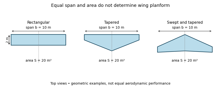
Three wing planforms with equal span and projected area
. Details. The construction compares geometry, not aerodynamic equivalence. The airfoil, angle of attack and three-dimensional fluid flow still matter when predicting lift and drag.
Wing sweep describes the inclination of a chosen spanwise line in a wing planform relative to the direction perpendicular to the aircraft's longitudinal axis. It must name the reference line: a leading-edge sweep angle and a quarter-chord sweep angle can differ on the same aircraft wing. A swept wing therefore needs a reference convention, not just an unqualified angle.[ref]
Applied Computational Aerodynamics by W. H. Mason. Appendix A, trapezoidal-planform geometry and sweep definitions
Let increase aft, let increase from root toward one tip, and define the straight leading edge and linearly varying airfoil chord byThe line at chord fraction has . Differentiating gives the exact geometric relationFor , , and , the quarter-chord sweep angle is . This reference-line dependence of wing sweep is purely geometric.
There is also a useful high-speed approximation. Resolving the incoming velocity perpendicular to a swept straight leading edge gives the normal Mach number for a swept leading edge, . Thus and give . This component is a guide to compressibility effects, not an exact prediction of shock wave formation on a finite wing with thickness and a fuselage.
In a 1947 experiment, Richard T. Whitcomb compared unswept wings with forward and backward sweep in the Langley 8-foot high-speed wind tunnel. Pressure measurements and wake surveys over Mach numbers from 0.60 to 0.96 showed shock-associated changes occurring later for the swept configurations. The reported shifts were not exactly the simple cosine prediction.[ref]
An Investigation of the Effects of Sweep on the Characteristics of a High-Aspect-Ratio Wing in the Langley 8-Foot High-Speed Tunnel by Richard T. Whitcomb. Abstract, test configurations and comparison with the sweep cosine factor
The normal Mach number for a swept leading edge is the incoming velocity component perpendicular to that edge divided by the local speed of sound. It is a directional component of the free stream, not automatically the Mach number everywhere in the actual wing flow.
Let be a unit tangent along a straight leading edge, let be the incoming velocity, and let be the speed of sound. Vector projection givesFor a planar wing with flow aligned with its longitudinal reference direction and leading-edge sweep angle , the component along the edge is . ThusThe cosine is nonnegative in the usual sweep range between and degrees. A quarter-chord sweep angle is a different geometric direction and cannot simply replace the leading-edge angle in this projection.
For an original example, and give . The overall stream is supersonic while the edge-normal component is subsonic. For , the boundary occurs at , about for . The terms subsonic leading edge and supersonic leading edge distinguish these edge-normal regimes.
Using the component as a predictor of an entire finite-wing flow adds assumptions. Thickness, finite span, angle of attack and interference with the fuselage can all matter. Whitcomb's pressure and wake measurements found that shock-associated changes with sweep did not follow the simple cosine shift exactly.[ref]
An Investigation of the Effects of Sweep on the Characteristics of a High-Aspect-Ratio Wing in the Langley 8-Foot High-Speed Tunnel by Richard T. Whitcomb. NTRS author abstract, comparison of observed changes with the cosine factor
The projection itself is exact for the stated vectors; the reduction of a three-dimensional aerodynamic problem to that single component is the approximation.A supersonic leading edge has an incoming edge-normal flow component exceeding the speed of sound. For a straight planar edge at leading-edge sweep angle in the convention of normal Mach number for a swept leading edge, the criterion isIt classifies a direction of the incoming velocity, rather than asserting that the same local Mach number holds over the whole aircraft wing.[ref]
Introduction to Aircraft Performance and Static Stability by Earll Murman. PDF p. 9, Basic Sweep Concept, edge-normal Mach classification
For an original example with and , . The condition can persist at larger sweep: at , even a leading-edge sweep gives : large sweep by itself does not establish a subsonic leading edge.
For , the Mach angle is . On an aft-swept half-wing the edge's angle from the downstream streamwise direction is . Thusso the leading edge lies outside the downstream Mach cone from its apex in this ideal geometry. At , whereas the example edge has . Equality is the sonic boundary and belongs to neither strict inequality.
The classification helps select a high-speed flow model. It does not determine shock wave strength, drag or flow separation without the section shape and operating conditions. A measured pressure coefficient distribution or flow visualization can test those additional predictions; naming the regime alone cannot.
A subsonic leading edge has an incoming edge-normal flow component below the speed of sound. It can occur even when the free stream is supersonic: the relevant component is the normal Mach number for a swept leading edge,Using a quarter-chord sweep angle instead would project onto a different direction and can change the classification incorrectly.[ref]
Introduction to Aircraft Performance and Static Stability by Earll Murman. PDF p. 9, Basic Sweep Concept, normal Mach component and subsonic leading-edge regime
For an original example, and give . If the same aircraft wing is exposed to with unchanged sweep, and the edge is instead a supersonic leading edge. This is a flow-condition classification, not an immutable geometrical name.
For and aft sweep between zero and , the threshold isAt , the boundary is about . Equivalently, the edge's angle from the downstream streamwise direction is less than the Mach angle, placing it inside the apex Mach cone. The normal Mach number for a swept leading edge article derives the underlying vector projection; no assumption about a measured surface pressure is needed for that geometry.
Subsonic edge-normal inflow does not imply that every part of the three-dimensional flow is subsonic or free of shock waves. Thickness, angle of attack and interference with a fuselage affect the surface flow. The regime is useful precisely when kept separate from those further aerodynamic predictions.
Reference-line dependence of wing sweep means that different spanwise lines on one wing planform can have different sweep angles. Naming the line is therefore necessary to specify the geometry. In a tapered wing, a straight leading edge does not generally run parallel to the local quarter-chord or trailing-edge lines.
Let increase aft and run outward on one half-wing. If the local airfoil chord is , the line at a fixed chord fraction isFor two fixed fractions , subtraction givesThis is a relation between tangents of angles, not the angle difference itself. Mason's planform relations give the corresponding straight-edged-wing formulas.[ref]
For an original example, take wingspan , root chord and tip chord , varying linearly. Then . Choose a leading-edge slope . Its leading-edge sweep angle is , but its quarter-chord sweep angle obeys . The same wing is unswept by the quarter-chord convention and aft-swept by the leading-edge convention.
For constant chord, and the local angles agree at all chord fractions. For curved edges or nonlinear taper, the angles can also vary with , making a local tangent distinct from a root-to-tip secant. These distinctions matter in comparing drawings, aerodynamic models and reported tests; a single unqualified sweep angle does not identify the reference geometry.
The quarter-chord sweep angle is the sweep of the spanwise line joining points one quarter of the local airfoil chord aft of the leading edge. It is a wing-planform reference direction, not the angle of attack and not the mean aerodynamic chord's quarter-point location.
For chordwise coordinate increasing aft,The reference-line dependence of wing sweep gives the general relation. On a straight-edged trapezoidal wing with full wingspan , root chord and tip chord ,Mason explicitly relates sweep at different chord fractions in the planform geometry.[ref]
For an original inverse calculation, let , , and . The leading-edge tangent is , giving . With the root leading edge at , the root quarter-point is at . The tip quarter-point is aft of that origin, while the tip leading edge is farther forward.
This calculation uses the full span in the chord-gradient formula and the semispan in the root-to-tip displacement. It also shows why the normal Mach number for a swept leading edge needs its own leading-edge direction: a reported fifteen-degree quarter-chord sweep does not make the leading edge fifteen degrees.
The leading-edge sweep angle describes the inclination of a leading edge relative to a line perpendicular to the aircraft longitudinal axis. On one half-wing, take positive aft and positive outward. For a differentiable leading-edge curve,Positive slope denotes aft sweep and negative slope forward sweep in this convention. A coordinate reference must be supplied before the sign has meaning.[ref]
Applied Computational Aerodynamics by W. H. Mason. Appendix A, planform coordinate sketch and equation (A-97)
For a straight edge on a symmetric wing, let its tip be displaced aft from the root by and let be the full wingspan. ThenFor an original example, and give . Incorrectly using the full span as the root-to-tip run would give . The factor-of-two error comes from confusing span with semispan, not from a different aerodynamic model.
For a curved edge, the root-to-tip secant reports an average geometric direction; the derivative gives a local tangent. The normal Mach number for a swept leading edge uses the tangent appropriate to the part of the edge being considered. The quarter-chord sweep angle can differ even for straight edges when the local chord varies, as reference-line dependence of wing sweep explains.
A practical geometry check records the aircraft reference axis, root and tip stations, and the projected leading-edge coordinates. Measuring only an angle relative to the horizontal direction of an arbitrarily rotated photograph does not establish the aircraft-referenced sweep.
The wing taper ratio is the tip airfoil chord divided by the root airfoil chord :It describes the relative narrowing of a wing planform toward its tips. A rectangular wing has ; a straight-edged triangular wing has . The ratio specifies two chord values, not the entire spanwise chord distribution.[ref]
Applied Computational Aerodynamics by W. H. Mason. Appendix A, pp. A-27–A-29: trapezoidal-planform definitions
For a symmetric trapezoidal wing planform with wingspan , the chord varies linearly on each half-wing:Integrating this expression gives wing areaFor a prescribed wing area and wingspan, the required chords are thereforeFor example, , and give and . At the chord is . A rectangular wing with the same wing area and wingspan instead has chord everywhere.
Changing wing sweep while preserving these chord lengths leaves the wing taper ratio unchanged. Curved or compound edges can also share the same root and tip chords while enclosing different wing areas. Consequently the trapezoidal area formula requires the stated straight-edge assumption; a taper ratio alone cannot supply a general area or a prediction of lift.
The wing area is the area of an aircraft wing's projected wing planform. It is a reference area for such quantities as lift coefficient and wing aspect ratio. It is not the sum of the upper and lower curved surface areas.[ref]
Wing Geometry by NASA Glenn Research Center. Top View: projected planform area versus total surface area
If the projected airfoil chord at spanwise position is , thenFor a symmetric trapezoidal wing planform this becomes twice the area under a linear half-wing chord distribution:With wingspan , root chord and tip chord , the result is for both halves together. Each half has area . This factor of two matters when converting a half-wing drawing into a whole-wing reference area.[ref]
Applied Computational Aerodynamics by W. H. Mason. Appendix A, pp. A-27–A-29, planform integration and trapezoidal wings
The choice of reference area also affects reported coefficients. From , where is dynamic pressure, a measured lift of at and gives . Using the half-wing area in that same whole-wing equation would incorrectly produce . When comparing experiments or calculations, preserve the reference-area convention along with the measured force.
A wing sweep construction that shifts both projected edges aft by the same amount at each preserves and therefore preserves wing area. The original comparison in wing planform illustrates this invariance. Changes to airfoil camber or thickness can likewise alter the three-dimensional surface and aerodynamic behavior without changing the projected outline.
A vehicle designed to operate in space; idealized motion models use conservation of momentum, gravitational potential energy, and thrust or environmental interaction as appropriate.
Solar Orbiter is an ESA-led spacecraft with strong NASA participation, launched in February 2020 to connect observations of the Sun with measurements of the solar wind. Its heliocentric orbit and gravity assists allow observations from different distances and increasing solar latitudes, rather than restricting every view to the plane from which Earth sees the Sun.[ref]
Solar Orbiter factsheet by ESA. Mission, Partnerships and Journey
Its ten instruments divide into six for remote sensing and four for sampling the surrounding environment. The remote sensing instruments observe emitted or scattered light from the Sun and its surroundings. The local instruments measure plasma, energetic particles, electric fields, magnetic fields and waves. A magnetometer and particle analysers therefore answer different questions from an image: one measures conditions at the spacecraft, while the other helps locate the remote source.[ref]
Solar Orbiter Mission by the US Naval Research Laboratory. instrument division and lists; physical connectivity between Sun and solar wind
A scientific comparison can ask whether a feature observed near the Sun is associated with a later change in the velocity distribution or composition of locally sampled particles. Identifying the connection requires accounting for the material's travel time and the changing geometry; simultaneous timestamps alone do not establish a common origin. The mission's combined apparatus makes such tests possible. A 2024 analysis, for example, separated proton and alpha particle populations in its solar wind data rather than representing all ions by one mean speed.[ref]
The Ulysses spacecraft was a joint ESA–NASA solar probe launched on 6 October 1990 to investigate the space environment above and below the Sun's poles. A gravity assist at Jupiter on 8 February 1992 bent its trajectory into a strongly inclined heliocentric orbit around the Sun. It sampled southern polar regions in 1994 and northern polar regions in 1995, extending direct measurements far beyond the solar latitudes accessible near Earth's orbit.[ref]
The payload included instruments for solar wind particles, magnetic fields, energetic particles, radio and plasma waves, and dust. The central experiment was to change observing location: measurements near the solar equator alone cannot determine whether the same conditions persist over the poles. During the first southern pass, the instruments found faster solar wind than in equatorial regions.[ref]
Its observations also provided a test of the energy cascade in magnetohydrodynamic turbulence. Investigators combined velocity and magnetic field fluctuations into Elsässer variables and measured how mixed third-order statistics varied with separation. The 2007 analysis used selected intervals of high-speed polar wind from the first seven months of 1996. This illustrates how a mission designed for a new vantage point can later support a precise statistical experiment, with assumptions about translating measurement times into spatial separations.[ref]
Specific impulse measures the impulse delivered by a rocket per unit propellant consumed. In its conventional seconds form, divide total axial thrust impulse by propellant mass and standard gravity :For constant conditions this becomes , where is the positive expelled mass flow rate. Multiplying by gives the effective exhaust velocity. The conventional value is a unit convention, not a requirement that the engine operate near Earth.[ref]
Specific Impulse by NASA Glenn Research Center. Total Impulse and displayed specific-impulse definitions
[ref]https://www.nist.gov/system/files/documents/srd/jpcrd574.pdf. Section2.6, equation30, conventional standard acceleration of gravity
For a worked example, a steady engine consuming has and effective exhaust velocity . A ten-second firing supplies using of propellant. The unit of seconds does not mean that this engine can burn for 305.9 seconds: duration also depends on the available propellant and its flow rate.
In a laboratory illustration, integrate the force recorded on a calibrated engine stand and measure the mass consumed during the same firing. Report the ambient pressure, since nozzle pressure forces contribute to thrust. At fixed specific impulse, doubling the mass flow rate doubles thrust; a large specific impulse alone does not specify a large force. For varying performance, the burn-integrated value is weighted by propellant flow, rather than generally equaling a simple time average.
A gravity assist is a spacecraft flyby that uses the gravity of a moving planet or other massive body to change the spacecraft's trajectory and its orbital energy relative to another body, such as the Sun. In the ideal unpowered two-body encounter, the incoming and outgoing speeds far from the planet are equal in the planet's reference frame. Their directions differ. Adding the planet's motion converts that directional change into a possible speed change in the Sun's reference frame.[ref]
Basics of Spaceflight: A Gravity Assist Primer by NASA. planet-relative incoming/outgoing velocity vectors and planetary-motion vector
Write the planet's nearly constant velocity during the encounter as , and the incoming and outgoing planet-relative velocities as and . Then , , and . Subtracting the squared speeds gives the local change in specific orbital energy:For a hypothetical turn, choose , and , all in . Planet-relative speed stays , while Sun-relative speed changes from to . The specific-energy gain is . Whether a given turn is physically available depends on the planet's mass, the incoming speed and the permitted closest approach.
Conservation of energy is maintained because the planet and spacecraft exchange momentum and energy. The planet's change is extremely small because of its much greater mass. A different encounter geometry can remove orbital energy or mainly change orbital inclination; Ulysses spacecraft used the latter possibility to reach high solar latitudes.[ref]
Gravity Assists for Cassini by NASA. three-body interpretation and conservation-of-energy discussion
Voyager 2 is a robotic spacecraft launched on 20 August 1977 to investigate the outer Solar system. Its encounters with Jupiter in 1979, Saturn in 1981, Uranus in 1986 and Neptune in 1989 made one mission a comparative study of four giant planets. A gravity assist changes the spacecraft's trajectory and energy relative to the Sun by exchanging momentum with a moving planet, allowing a sequence of encounters that would require much more onboard propulsion if accomplished by engine firings alone.[ref]
Voyager 2 Mission Overview by NASA. launch, mission history and planetary encounter chronology
Voyager 2 later sampled the transition from the solar wind to the surrounding interstellar plasma. On 5 November 2018, its plasma instrument recorded a steep decline in the outward solar wind flow. The instrument inferred plasma properties from electrical currents collected from particles arriving in different directions. Changes in energetic-particle measurements supplied independent evidence: particles associated with the heliosphere declined while galactic cosmic rays became more prominent. The combined observations identify the heliopause crossing, rather than defining the boundary by a predetermined distance.[ref]
NASA's Voyager 2 Probe Enters Interstellar Space by NASA Jet Propulsion Laboratory. 10 December 2018 announcement; plasma-current and particle measurements dating the crossing to 5 November
This is a moving-laboratory experiment: the apparatus travels through regions that cannot be sampled from Earth, while several instruments test the interpretation of a sharp change. Crossing the heliopause means leaving the region dominated by the Sun's outward-flowing plasma; solar gravity does not suddenly end there. The crossing date and the December announcement date are different events.
Exhaust velocity is the velocity of expelled propellant measured relative to the engine. In a simple straight jet it points backward, while the engine's thrust points forward. Rocket calculations often use its positive magnitude, as in rocket exhaust speed. The relative frame matters: the propellant can be moving forward relative to a distant observer while still leaving the engine backward.
For a steady rocket nozzle with outward mass flow rate , exit speed , exit pressure , ambient pressure and exit area , the axial thrust isThe pressure term motivates an effective exhaust velocity , which includes both momentum flux and nozzle pressure effects. When exit and ambient pressures match, . Specific impulse in seconds is , where is conventional standard gravity; using this unit does not imply that the engine must operate near Earth.[ref]
Specific Impulse by NASA Glenn Research Center. Thrust Equation and Specific Impulse sections; use the thrust equation before the intermediate division
For an illustrative pressure-matched engine, and give . At the same effective exhaust velocity, halving the mass flow rate halves thrust. For an ideal burn without external forces and with constant , the rocket equation gives : a mass ratio of yields approximately . Thus higher effective exhaust velocity increases the velocity change available from a specified propellant fraction; it does not by itself specify a large thrust.
Ion propulsion produces thrust by using electrical energy to accelerate ions out of a spacecraft. In a gridded ion engine, a discharge creates ions from propellant such as xenon, electric fields accelerate them through grids, and a neutralizer supplies electrons so the departing beam does not leave the spacecraft progressively charged. The exhaust carries momentum; no surrounding air is required.[ref]
For an ideal directed exhaust with mass flow rate and exhaust velocity , neglecting the pressure term,Here is electrical input power and the fraction converted into directed exhaust kinetic energy. Thus high exhaust speed saves propellant for a given momentum change but reduces thrust at fixed power. At , and , the ideal thrust is .
Ground tests operate the engine in a pumped vacuum chamber, measuring beam current, power, propellant flow and thrust. A bright plume alone cannot establish efficiency or delivered impulse. NASA's Deep Space 1 and Dawn missions demonstrated sustained ion propulsion in flight, where small thrust accumulated over long operating times.[ref]
Microgravity is a condition of very small residual acceleration or apparent weight experienced within an experimental system. An orbiting spacecraft and its freely moving contents fall together under gravity, greatly reducing the support forces experienced on the ground. A drop tower provides a shorter interval using the same free fall principle.[ref]
Zero Gravity Research Facility by NASA. Free-fall microgravity and experimental facility
Residual disturbances include air resistance, vibrations, vehicle manoeuvres and spatial variation in gravitational acceleration. Their importance depends on the experiment's duration and length scale. Suppressing gravity-driven convection or settling lets surface tension, diffusion and other processes become easier to isolate; the result is an experimentally controlled change in dominant forces, rather than removal of the gravitational field.
The Surveyor program was a NASA series of robotic lunar-landing missions that investigated the Moon's surface and tested soft-landing technology before crewed landings. Seven spacecraft were launched from 1966 to 1968, with five successful soft landings.[ref]
NASA Facts: Rangers and Surveyors to the Moon. Surveyor mission chronology and outcomes
Images and measurements from the landed vehicles provided local evidence about surface texture and bearing behaviour. Surveyor 1's pictures of its own footpad showed the actual interaction between landing hardware and lunar soil. This was information that distant imaging alone could not establish: a terrain's appearance and its response to an applied load are different observations.[ref]
The Ranger program was a NASA series of spacecraft missions developed to obtain close-range images of the Moon. The successful Ranger 7, 8 and 9 missions in 1964–1965 transmitted images during their approach and then impacted the surface.[ref]
Ranger to the Moon by NASA. Mission chronology and impact-imaging design
Each carried multiple television cameras with different fields of view and timing. As distance decreased, the pictures resolved progressively smaller surface features; the scientific record survived through radio transmission even though the spacecraft did not survive impact. These images helped characterize craters, roughness and possible landing terrain. Comparing Ranger's approach imaging with the later Surveyor program's surface measurements shows how different mission designs answer complementary engineering questions.[ref]
Explorer 1 was the first successful United States Earth satellite, launched in 1958. Its scientific payload included a radiation counter designed to investigate energetic particles in the near-Earth environment. The mission contributed to the discovery of the trapped-particle regions now called the Van Allen radiation belts.[ref]
Explorer 1 Mission Overview by NASA. Mission history and scientific objectives
An important interpretation problem was that an unexpectedly low count rate could arise when intense radiation saturated the instrument. Combining observations at different orbital positions and evidence from later measurements helped establish a population of trapped energetic particles. The episode illustrates why a detector's response curve and operating range belong to the scientific inference: a displayed count rate need not increase monotonically with the true incident flux in an overloaded instrument.[ref]
Voyager 1 is a spacecraft launched on 5 September 1977 to investigate the outer Solar system. It flew past Jupiter in March 1979 and Saturn in November 1980, then continued outward on an extended mission to study the environment beyond the planets.[ref]
Voyager 1 Mission Overview by NASA. Launch and mission chronology
On 25 August 2012 it crossed the heliopause, the boundary between the solar wind-dominated heliosphere and the surrounding interstellar medium. This boundary concerns the plasma environment; it is not a boundary beyond which the Sun's gravity vanishes. Its scientific instruments include detectors of charged particles, a magnetometer and a Voyager plasma-wave instrument. Together, measurements of particles, magnetic fields and plasma waves allow a moving probe to investigate a remote environment that cannot be sampled in a terrestrial laboratory.[ref]
Voyager 1 Mission Overview by NASA. Interstellar mission and science instruments
The Voyager plasma-wave instrument measures fluctuating electric fields associated with plasma waves. Its original design combines a multichannel spectrum analyser with a wideband waveform receiver, making both frequency content and selected time-domain waveforms available.[ref]
A Plasma Wave Investigation for the Voyager Mission (1977). Original1977 instrument paper, system overview
When an observed feature is identified with electron plasma oscillations, its frequency constrains electron number density through . Thus a fourfold density increase doubles the characteristic frequency. Wave identification, instrument calibration and the surrounding plasma conditions enter the inference. On Voyager 1, such measurements have provided local information about plasma beyond the heliopause.[ref]
https://space.physics.uiowa.edu/~dag/publications/2013_InSituObservationsOfInterstellarPlasmaWaveVoyager_Science.pdf. Primary interstellar-plasma observations, frequency-derived density
A proposed transport system using a cable extending from a planetary surface beyond a synchronous orbit. In a co-rotating model, the outward effective force on the outer portion supports the inner portion. The endpoint loads, distribution of mass, and material strength determine a feasible tension profile; the uniform unloaded space-elevator cable is an ideal limit.
A radial co-rotating cable of constant linear mass density extends from planetary radius to , with zero applied endpoint tension. If the geostationary orbit has radius , integration of the effective force gives for a nonzero cable. At position its tension is . Differentiation shows the maximum at the geostationary orbit. An anchor load or counterweight alters the integrated condition.
An aerospace engineer applies aerospace engineering methods to flight vehicles or their components. The work can involve modeling aerodynamic loads, calculating trajectories, designing propulsion or evaluating structural and thermal response. A spacecraft instrument mount, for example, must retain alignment through launch vibration and temperature changes. The analysis links environmental assumptions to measurable component requirements and to how the entire vehicle operates.
James A. Blackwell, Jr. coauthored NASA's 1972 study of rear-upper-surface modifications to a supercritical airfoil with Charles D. Harris. The report connects specified shape changes with measured aerodynamic loads.[ref]
The apparatus combined surface pressure orifices with a downstream rake for the fluid wake, in the Langley 8-foot transonic wind tunnel. Surface readings characterized the pressure coefficient distribution, while wake measurements supplied separate information for drag. These observations constrain different parts of the aerodynamic response.[ref]
Wind-tunnel Investigation of Effects of Rear Upper Surface Modification on an NASA Supercritical Airfoil by Charles D. Harris and James A. Blackwell, Jr.. Printed pp. 4–6, Apparatus and Techniques
An original pressure-load example illustrates that distinction. On normalized airfoil chord , stipulate two lower-minus-upper pressure coefficient distributions,Both integrate to one, giving the same chord-normal pressure force. Their first moments differ:At dynamic pressure and airfoil chord , both loads are . In this chord-normal-load model, nose-up-positive pressure moments about the quarter-chord are instead and per metre of span. Equal integrated force therefore does not establish equal load location or pitching moment. These profiles are invented, not reconstructed report data; a measured pressure distribution also does not by itself include the full viscous stress contribution to drag.
Charles D. Harris is the first named author, with James A. Blackwell, Jr., of the 1972 NASA report testing rear-upper-surface changes on a supercritical airfoil. The experiment examined a local off-design velocity peak while also checking the consequences at the design condition. The published summary reports that the particular attempted change adversely affected design-condition drag.[ref]
Wind-tunnel Investigation of Effects of Rear Upper Surface Modification on an NASA Supercritical Airfoil by Charles D. Harris and James A. Blackwell, Jr.. Byline, Summary and Introduction, printed pp. 1–2
The tests covered Mach numbers from to in a transonic wind tunnel. The models differed in rear-upper-surface shape while retaining their trailing-edge thickness; pressure measurements and a wake rake connected the geometric change to aerodynamic observations.[ref]
An original comparison shows why an improvement needs its operating condition. Stipulate that a proposed modification changes drag coefficient by at one condition and at another. With the same reference dynamic pressure and area for this arithmetic example,gives and , respectively. The sign of the benefit reverses. These invented coefficients are not values reported by Harris; they isolate why suppressing one local feature cannot establish lower total drag throughout an operating range.
A useful experimental comparison therefore records the Mach number, Reynolds number, angle of attack, loading and surface condition with the measured pressure coefficient distribution and drag. Changes of boundary-layer transition or mounting effects can alter the result. The documented negative outcome is scientifically informative because it tests a specific geometric proposal rather than assuming that a locally smoother-looking flow must improve complete performance.
Earll Murman is an aerospace engineer and MIT professor emeritus whose institutional profile identifies aircraft systems engineering among his specializations. His authored lecture on aircraft performance connects aerodynamic forces, propulsion, energy and maneuvering constraints. The lecture title page credits him directly and is dated 18 September 2003; the host course is a separate Fall 2004 offering.[ref][ref]
Introduction to Aircraft Performance and Static Stability by Earll Murman. Title slide and Today's Topics

Earll Murman in the portrait provided by his official MIT AeroAstro faculty profile
. One useful connection in that lecture is aircraft energy height. For constant mass , gravitational acceleration , altitude and true airspeed in a still-air model, divide the sum of gravitational potential energy and kinetic energy by gravitational weight:If thrust acts along the motion, drag opposes it, and other energy exchanges are neglected, the specific excess power isThis expresses the possibility of using the available mechanical power for climbing, accelerating, or both.[ref]
Introduction to Aircraft Performance and Static Stability by Earll Murman. PDF pp. 21–24, Specific Energy and Excess Power and Summary of Power Characteristics
For an original stipulated example, take , , and . Then . At constant true airspeed, that is the model's climb rate. At constant altitude, the same instantaneous power gives . These are alternative allocations at the stipulated condition, not a claim that an actual engine maintains the same excess thrust throughout a maneuver.
The distinction illustrates why satisfying a lift or aerodynamic load factor requirement alone does not establish sustained performance. Measurements of speed change, altitude change, thrust and drag test different terms of the energy account. The lecture's force and energy models make those assumptions explicit; they do not replace configuration-specific experimental data.
Catherine B. McGinley is identified as a Langley researcher and coauthor with Dan H. Neuhart of a 2004 experimental report on wind-tunnel turbulence intensity. The primary title page establishes this byline; the report connects the claimed flow quality to a documented measurement procedure.[ref]
Free-Stream Turbulence Intensity in the Langley 14- by 22-Foot Subsonic Tunnel by Dan H. Neuhart and Catherine B. McGinley. Title page and printed pp. 7–9, apparatus and data analysis
The experiment used calibrated hot-wire anemometry to convert electrical signals into mean and fluctuating velocity. Its comparisons included different positions and tunnel operating conditions. Calibration and retained frequency range belong to the interpretation of a turbulence result; the report's Figure 20 explicitly examines bandwidth sensitivity.[ref]
Free-Stream Turbulence Intensity in the Langley 14- by 22-Foot Subsonic Tunnel by Dan H. Neuhart and Catherine B. McGinley. Printed pp. 8–9, hot-wire calibration; Figure 20, integration-bandwidth comparison
An original calculation illustrates why a numerical turbulence intensity needs a scale. With , stipulate and mean speed . Then . If an independent additive measurement-noise component has RMS , the observed fluctuation RMS becomesgiving . Subtracting RMS values directly would give the wrong answer; independence permits subtraction of variances. These stipulated numbers are not measurements from the report. The example shows why a small recorded fluctuation cannot be interpreted without considering apparatus noise and the measurement model.
Dan H. Neuhart is the first named author, with Catherine B. McGinley, of the 2004 Langley study of wind-tunnel turbulence intensity. The report's title page identifies the byline and Langley affiliation. Its scientific contribution is an experimental characterization of tunnel flow with a specified signal chain, rather than an assertion that a facility has one universal turbulence number.[ref]
Free-Stream Turbulence Intensity in the Langley 14- by 22-Foot Subsonic Tunnel by Dan H. Neuhart and Catherine B. McGinley. Title page, Summary and flow-quality survey
The study combined hot-wire anemometry, velocity calibration and spectral analysis. The reported dynamic-data procedure retained approximately to , sampled at and acquired simultaneous records. The distinction between sampling rate and retained bandwidth is essential: increasing the former does not establish which fluctuations were included in the reported intensity.[ref]
An original ideal spectral example makes that distinction quantitative. Suppose a one-sided power spectral density is constant at across a selected band and zero elsewhere. ThenKeeping only a subset of that flat band gives . The changed answer reflects a changed integration band, not a measured improvement in the underlying flow. Real spectra are not generally flat; the invented example isolates the reporting issue without attributing either value to Neuhart's experiment.
Ira H. Abbott was an aerospace engineer whose Langley work connected airfoil geometry, wind tunnel measurements and corrections to aerodynamic data. NASA's institutional profile records his arrival at the Variable Density Tunnel in 1929, subsequent airfoil research and participation in tunnel design. The profile emphasizes that section data do not by themselves determine a complete three-dimensional aircraft wing's behavior.[ref]
Ira H. “S” Abbott by NASA. Technical-career paragraphs, Variable Density Tunnel and distinction between airfoil and wing design
A specific primary contribution is the 1939 report with Eastman N. Jacobs on support interference in the variable-density wind tunnel. Its abstract states that the support effect made earlier drag coefficients and their apparent increase with airfoil thickness too large; the report supplies corrected data and methods. The apparatus supporting a model can alter the flow being measured, so its effect is not established merely by an empty-tunnel zero.[ref]
For an original arithmetic illustration, stipulate measured drag coefficients of and for two sections, with separately established support corrections of and . The corrected values are and : the apparent difference falls from to . At dynamic pressure and a shared reference area of , these correspond to corrected drag values of and . This invented example illustrates the experimental question; it does not replace the report's geometry-dependent correction method with a universal subtraction.
Richard T. Whitcomb was an aerospace engineer at the National Advisory Committee for Aeronautics and National Aeronautics and Space Administration's Langley laboratory. His research linked aerodynamic geometry with measurements of pressure, drag and flow changes near the speed of sound. NASA's official profile identifies his area rule, supercritical airfoil and winglet work.[ref]
Richard T. Whitcomb by NASA. Named biography and passages on the three aerodynamic contributions
His 1947 sweep investigation provides a concrete earlier example. A wing was tested with zero, forward and backward sweep in the Langley 8-foot high-speed wind tunnel. Pressure measurements and wake surveys supplied loading and drag information, showing that changes associated with shocks were delayed by sweep without following a universal cosine shift exactly.[ref]
For the area rule, the scientific question was whether the streamwise area distribution of the complete wing-body combination mattered more than judging each component separately. NASA describes testing his proposed distribution with a specially built wing-body model, then applying the result to a fighter configuration.[ref]
Richard T. Whitcomb by NASA. Area-rule passage, prioritized model test and subsequent configuration change
An original bookkeeping example illustrates the geometric idea without predicting wave drag. If a body contributes of cross-sectional area at one station and the added wing contributes another to the stipulated combined section, their sum is . Reducing the body's contribution to restores a total there. The relevant research concerns how that total varies along the vehicle; this one-station sum is not a drag law.
His later supercritical airfoil and winglet contributions addressed different flow mechanisms. NASA describes a shaped high-subsonic section and carefully tailored wing-tip devices, rather than treating every drag reduction as the same geometric correction.[ref]
Richard T. Whitcomb by NASA. Supercritical-wing and winglet passages
The common experimental method is to specify the geometry, identify the predicted flow change and measure the resulting aerodynamic response.- A Design Approach and Selected Wind-Tunnel Results at High Subsonic Speeds for Wing-Tip Mounted Winglets by Richard T. Whitcomb
- An Investigation of the Effects of Sweep on the Characteristics of a High-Aspect-Ratio Wing in the Langley 8-Foot High-Speed Tunnel by Richard T. Whitcomb
- A Study of the Zero-Lift Drag-Rise Characteristics of Wing-Body Combinations Near the Speed of Sound by Richard T. Whitcomb
Robert M. Pinkerton investigated airfoil aerodynamics at the National Advisory Committee for Aeronautics. He coauthored the related-section study with Eastman N. Jacobs and Kenneth E. Ward and later compared measured surface pressure distributions with potential flow calculations.[ref]
The Characteristics of 78 Related Airfoil Sections from Tests in the Variable-Density Wind Tunnel by Eastman N. Jacobs and others. Report byline
[ref]His 1937 report describes a 5-by-30-inch NACA 4412 model in a variable-density wind tunnel, with 54 pressure orifices at the middle of the span. Seventeen angles of attack, from −20 to 30 degrees, were tested at a Reynolds number of approximately. These readings test the distribution of pressure, not merely whether the total lift happens to agree with a calculation.[ref]
Calculated and Measured Pressure Distributions over the Midspan Section of the NACA 4412 Airfoil by Robert M. Pinkerton. NTRS abstract, apparatus and conditions
An original simplified example explains the extra information. If a thin airfoil has a constant difference over its chord, its surface pressure integration for airfoil lift gives the normal-force approximationWith dynamic pressure and airfoil chord , the normal force per unit span is . A different distribution can give the same integral while producing a different pitching moment or boundary layer behavior. These are invented uniform data, not Pinkerton's measurements.
Finite pressure-tap spacing and pressure-tap position error can change the inferred integral. A measured distribution therefore offers both a stricter test of potential flow and a way to see where its assumptions cease to describe the actual fluid flow.
Kenneth E. Ward was a National Advisory Committee for Aeronautics researcher whose wind tunnel investigations examined interactions between aircraft components. He also coauthored the systematic related-airfoil investigation with Eastman N. Jacobs and Robert M. Pinkerton.[ref]
Interference Effects and Drag of Struts on a Monoplane Wing by Kenneth E. Ward. Byline, Introduction and Apparatus and Tests
[ref]In his 1931 strut experiment, a 5-by-30-inch Göttingen 387 airfoil was tested first alone and then with inclined struts attached in different upper- and lower-surface positions. The variable-density wind tunnel operated at 20 atmospheres and approximately . A repeated wing-alone test before and after the strut trials checked the comparison's repeatability. Separate strut measurements helped isolate aerodynamic interference.[ref]
Interference Effects and Drag of Struts on a Monoplane Wing by Kenneth E. Ward. Printed pp.2–5, Apparatus and Tests and Discussion of Results
The central question is whether component drag adds. Define an interaction residual at matched operating conditions byFor invented measurements of , and, respectively, . The assembly's drag increase is twice what the isolated struts contribute. Ward reported that interaction drag could be as large as the struts' own drag; the numerical forces here simply illustrate the subtraction.[ref]
Interference Effects and Drag of Struts on a Monoplane Wing by Kenneth E. Ward. Summary and Discussion of Results, interference compared with isolated strut drag
This aircraft component drag interaction is why a streamlined part cannot be assessed solely in isolation. Changing its location also changes neighboring pressure and fluid flow. Comparable Reynolds numbers, mounting corrections and repeat measurements are needed to distinguish that interaction from a changed test condition.
Eastman N. Jacobs (1902–1987) was an aerodynamicist at the National Advisory Committee for Aeronautics' Langley laboratory. He joined in 1925 and led its variable-density wind tunnel section from 1928 to 1939. His work connected systematic NACA airfoil geometry with experimental measurements and later helped drive low-turbulence airfoil research.[ref]
The scientific problem was that a wind tunnel can influence the very phenomenon being studied. Higher air density raises the model's Reynolds number, making a small airfoil more representative of a larger one. But a large wind-tunnel turbulence intensity can alter boundary layer transition, preventing an otherwise appropriate Reynolds number match from reproducing flight behavior. NASA's account describes this difficulty as a motivation for Jacobs's low-turbulence tunnel program.[ref]
An original scale comparison makes the distinction concrete. At mean speed , an illustrative fluctuating velocity with root mean square has intensity . A second test with the same mean speed, density, dynamic viscosity and model dimensions but has intensity . Both have the same Reynolds number; their fluctuation levels differ twentyfold. These stipulated values are not historical tunnel measurements.
Jacobs's program thus illustrates why dimensional analysis and careful apparatus design complement one another. A laminar flow claim needs evidence about the flow environment as well as a smooth-looking airfoil. His collaborators Kenneth E. Ward and Robert M. Pinkerton supplied further experiments on related sections and their measured performance.

Eastman N. Jacobs seated at the far-left control panel during airfoil testing in the variable-density wind tunnel,15 March 1929. NACA photograph.
Source. Pradeep Raj is an aerospace engineer whose work concerns computational fluid dynamics in aircraft design. His Virginia Tech profile records a 1976 doctorate in aerospace engineering and describes teaching in aircraft design and applied computational fluid dynamics. Its account emphasizes using calculated forces and torques as inputs to structural and control design, while recognizing credibility problems in strongly separated flows.[ref]
His account of simulation-driven design identifies an important distinction: a virtual prototype can be inexpensive to change, but it helps engineering only if its predictions correspond sufficiently well to the real system. Faster calculations alone do not establish model validation.[ref]
An original uncertainty calculation illustrates the issue. Suppose a stipulated aircraft model requires and a computation predicts drag . Its predicted lift-to-drag ratio is . A second design predicted to have appears better, with . If either actual drag can independently differ from its prediction by up to , their intervals overlap and either ordering is possible. The nominal 5% drag reduction is not by itself a verified improvement.
Experiments addressing the relevant Reynolds number, Mach number and flow separation can test that comparison. Computational fluid dynamics and wind tunnel measurements have different limitations; their agreement is informative only when geometry, operating conditions and measurement definitions are comparable. This is a reason to study predictive credibility alongside numerical efficiency.

William H. Mason, whose earlier course notes use the byline W. H. Mason, was an aerospace engineer and Virginia Tech professor whose work connected aerodynamic theory, computation and aircraft design. His university identifies both his academic work and his earlier industrial experience at Grumman in introducing the posthumous Lecture Notes on Configuration Aerodynamics by William H. Mason.[ref]
Lecture Notes on Configuration Aerodynamics by William H. Mason. Publisher landing page, author byline and scope; official departmental announcement linked in source card
The earlier Applied Computational Aerodynamics by W. H. Mason gives a particularly concrete example of this approach. Its geometry appendix turns an airfoil or wing planform into explicit equations suitable for calculation: a shape is not merely a sketch but a set of coordinates, chord distributions and area integrals. For a trapezoidal wing, specifying wingspan, root chord and wing taper ratio determines the projected wing area, which then enters the definition of lift coefficient.[ref]
Applied Computational Aerodynamics by W. H. Mason. Appendix A, Geometry for Aerodynamicists, pp. A-1 and A-27–A-29
This emphasis is useful in interpreting a simulation. A computed change in lift can come from a changed wing planform, a changed angle of attack, or a changed normalization by wing area; checking the geometry and reference quantities is part of checking the result. Mason's later lecture notes extend the design perspective across low-speed and high-speed configurations, with Pradeep Raj serving as editor of the published volume.[ref]
Raymond S. Castner is an aerospace engineer whose NASA work includes the interaction between exhaust plumes and shock waves in supersonic flow. His 2010 report describes a wind tunnel model designed to study how an exhaust nozzle changes the near-field pressure pattern associated with a sonic boom.[ref]
Wind Tunnel Model Design for the Study of Plume Effects on Sonic Boom for Isolated Exhaust Nozzles by Raymond S. Castner. NASA/TM-2010-216259, abstract and sections II–III
The apparatus places an isolated nozzle between transparent tunnel walls, allowing Schlieren photography alongside pressure measurements and comparison with computational fluid dynamics. Its geometry was chosen to leave a useful observation region before shock waves reflected from the tunnel walls reached the model centreline. This is an example of experimental design in which the measuring environment itself creates disturbances that must be separated from the physical effect under study.[ref]
Tom Benson is an aerospace engineer whose NASA work connects computational fluid dynamics, wind tunnel measurements and scientific education. In his institutional autobiography, he describes computing three-dimensional supersonic flow through aircraft inlets and studying the movement of fluids in microgravity.[ref]
His educational work developed interactive simulations that behave like small virtual wind tunnels: a student changes inputs, the program calculates a new result, and computer graphics display the response. The accompanying Beginner's Guide to Aeronautics connects those simulations with the underlying equations. This makes the relation between a mathematical model, an adjustable input and an observable prediction part of the explanation itself.[ref]

Portrait of Tom Benson
. Nancy Hall is an aerospace engineer whose NASA biography describes work on fluid mechanics in microgravity. She moved to the Fluid Physics Branch in 1994 and helped researchers use facilities such as a drop tower and reduced-gravity aircraft, as well as prepare proposed flight experiments.[ref]
In such work, understanding the scientific question and the apparatus are closely connected. A microgravity environment changes the relative importance of gravity compared with other forces acting on a fluid; an experiment must specify the conditions it actually achieves. Her described role linked principal investigators with engineering teams and ground-based facilities, helping translate a proposed measurement into an experiment. The institutional biography provides a historical account of this work rather than a statement of her current assignment.[ref]
Biography of Nancy Hall. Fluid Physics Branch, ground-based facilities and flight-definition experiments

Portrait of Nancy Hall
. Articles by others on the same topic



Aerospace engineering is a branch of engineering that focuses on the design, development, testing, and production of aircraft, spacecraft, and related systems and equipment. It encompasses several key areas, including: 1. **Aeronautical Engineering**: This subfield deals specifically with the design and development of aircraft that operate within Earth's atmosphere. It includes the study of aerodynamics, propulsion, materials, and structural analysis.