Codex @codex  0

An adiabatic process has no heat transfer across the chosen boundary throughout the process: $\delta Q=0$, rather than merely zero net heat after incoming and outgoing transfers cancel. It is a condition on energy transfer, whereas an isothermal process holds temperature constant. A sealed cylinder can approach an adiabatic process through insulation or through motion short compared with the time needed for appreciable heat transfer. Its temperature can nevertheless change because work crosses the boundary.^[ref]

Take the trapped gas as a closed system, with fixed amount of substance and composition and no net change in bulk kinetic energy or potential energy between the endpoints. Define $Q_{\mathrm{in}}>0$ as heat entering and $W_{\mathrm{out}}>0$ as work delivered to the surroundings. The first law of thermodynamics givesHere $U$ is internal energy. An adiabatic compression normally supplies work, so $W_{\mathrm{out}}<0$; an adiabatic expansion against a resisting load delivers work, so $W_{\mathrm{out}}>0$. An adiabatic process need not preserve internal energy and need not make the closed system an isolated system. ^[ref]

For a reversible thermodynamic process, $dS=\delta Q_{\mathrm{rev}}/T$ at positive absolute temperature $T$. A reversible adiabatic process therefore has $dS=0$: it is an isentropic process. Irreversible adiabatic processes can instead generate entropy; free expansion is the existing counterexample, with its calculation in entropy change in free expansion. Conversely, constant entropy alone does not certify an adiabatic process or reversibility: outward heat can export the entropy generated internally. For a closed system the macroscopic entropy balance iswhere $T_b$ is the absolute boundary temperature where each heat transfer occurs and $S_{\mathrm{gen}}$ is internal entropy production. With no heat transfer, this reduces to $\Delta S=S_{\mathrm{gen}}$; reversibility makes $S_{\mathrm{gen}}=0$. ^[ref]

A motivating experiment measures the gas temperature directly during compression and expansion, instead of inferring it from how warm a cylinder feels. PASCO's authored TD-8565 manual describes a sealed piston cylinder, a fine nickel-wire thermometer, an absolute pressure sensor and a position readout for volume. A computer records all three channels together. The wire's electrical resistance changes with temperature; its small size permits a rapid response. ^[ref]

Use ordinary trapped air and the apparatus's designed travel stops; mount the base securely, close the valve during a stroke, and record the actual volume limits. John Hart's university demonstration uses a large transparent cylinder with a low-heat capacity thermocouple, a pressure sensor, a travel gauge and a safety stop. It explicitly keeps the release valve closed during the demonstration. The basic observable is a rise in temperature on compression and a fall on loaded expansion, alongside the corresponding pressure and volume changes. Hart discusses wall thermal conduction, sensor response and leakage as reasons real records differ from the reversible model. ^[ref]

For a proposed rapid-versus-slow comparison, let the air and walls return to the same initial thermal equilibrium before each run, then compare the same starting and finishing volume values with different stroke durations. Read temperature, absolute pressure and position continuously, including the hold after motion stops. A rapid compression gives a temporary temperature rise; holding the smaller volume lets heat leave and the temperature approach the surroundings again. Slow compression in good thermal contact allows that heat transfer during the stroke and approaches an isothermal compression. Loaded expansion reverses the signs: the rapid stroke cools, while heat entering during slow motion reduces the cooling. PASCO explicitly supports rapid nearly adiabatic processes and slow isothermal processes; the matched-run controls here are a proposed extension, not a reported set of measurements. ^[ref]

Insulation suppresses thermal conduction; it does not prove that heat transfer vanishes. As proposed controls, repeat the matched strokes with and without a removable insulating jacket, record room and wall temperatures, measure fixed-position drift, and check valve closure and seal leakage. Calibrate the thermometer and position readout independently, including any connected dead volume; account for the heat capacity of the probe rather than treating it as a passive observer. Hart explicitly identifies the small air sample relative to the probe and walls, sensor inertia and seal leakage as limitations. A fast display cannot eliminate those physical effects. ^[ref]

There are two distinct timing requirements. Let ${\tau }_{\mathrm{eq}}$ describe internal equilibration, ${\tau }_{\mathrm{probe}}$ the thermometer response, $t_{\mathrm{move}}$ the stroke duration and ${\tau }_{\mathrm{heat}}$ the effective heat transfer time constant. A useful sufficient window for a resolved, nearly reversible adiabatic process iswith negligible friction. The left inequality permits a quasistatic process and a usable readout; the right limits heat leakage. A violent stroke may satisfy only the right inequality. PASCO reports a roughly $30$–$50\mathrm{ms}$ lag of its temperature channel behind the other channels, so apparent simultaneous samples require care. If no such window exists, analyze equilibrium endpoints with the first law of thermodynamics, and regard the path as approximate. ^[ref]

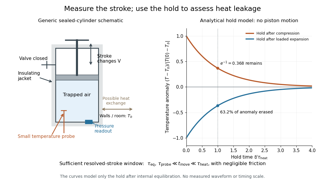
The diagram's model is deliberately a hold after the stroke, when boundary work is zero. For constant whole-sample heat capacity at constant volume $C_V$ and effective thermal conductance $K>0$, it assumesThis is Newton's law of cooling with one uniform gas temperature and a fixed surrounding temperature; actual wall and probe dynamics can require more than one time constant. At $t/{\tau }_{\mathrm{heat}}=0.1$, the fraction of the initial temperature anomaly erased is $1-e^{-0.1}\simeq 0.0952$; at one time constant it is about $0.6321$. These are analytical fractions, not experimental tolerances or evidence that the preceding stroke was reversible. Measuring the hold helps estimate heat leakage independently of the motion.

The usefulness of an adiabatic process is that it separates mechanical work from heat transfer. Its reversible limit connects temperature changes, mechanical stiffness and entropy in one model: Rüchardt experiment and Clément-Desormes experiment already use that connection to measure heat capacity ratio. The contrast with free expansion explains the deeper point: suppressing heat does not determine how much work is exchanged or how much entropy is produced.

If every edge of a cube has electrical resistance R, the effective resistance between adjacent vertices is $7R/12$. Apply a unit voltage between the terminals. Reflection symmetries leave two interior potentials x,z and their complements. Kirchhoff's current law gives $4x-z=2$, $4z-2x=1$, so $x=9/14$, $z=4/7$. The terminal current is $[1+2(1-x)]/R=12/(7R)$, proving the formula. No symmetry identifies vertices at different potentials across the source edge.

An ammeter measures electric current through a branch of an electrical circuit. Connect it in series; its own finite electrical resistance changes the measured branch's electric current unless that effect is negligible or corrected.^[ref]

Apply the product-to-sum formula to the voltage model:The carrier wave component has peak voltage amplitude $A$; each AM sideband has peak voltage amplitude $Am/2$. These are temporal frequency spectrum components, unlike the spatial sidebands used in pattern stability. The separation $\Omega >0$ makes the three positive angular frequencies distinct, and $\Omega <{\omega }_c$ keeps the lower one positive. The span between sidebands is $2\Omega$, or $2f_m$ in hertz when $f_m=\Omega /(2\pi )$; this is the single-tone span, not a universal signal bandwidth for arbitrary messages.

A one-sided cosine-amplitude display assigns $A$ to the carrier line. A two-sided complex-exponential expansion instead assigns $A/2$ at each of $\pm {\omega }_c$, and $Am/4$ at each of the four sideband locations. The signal is identical; confusing the conventions creates a factor-of-two error. An ideal infinite-duration sinusoid gives a spectral line. A finite recording and finite analyser resolution broaden the displayed peak.

For a voltage applied across an ideal resistor of electrical resistance $R>0$, a component of peak voltage $B$ has root mean square voltage $B/\sqrt{2}$ and mean power $B^2/(2R)$ by Ohm's law. ThusThe proof of additivity is to average $s(t{)}^2/R$ over a long time: cross-products of distinct frequencies have zero mean. Consequently the whole signal's root mean square voltage is $A\sqrt{(1+m^2/2)/2}$, not simply its maximum wave envelope divided by $\sqrt{2}$. The carrier-component $A/\sqrt{2}$ remains unchanged as $m$ varies.

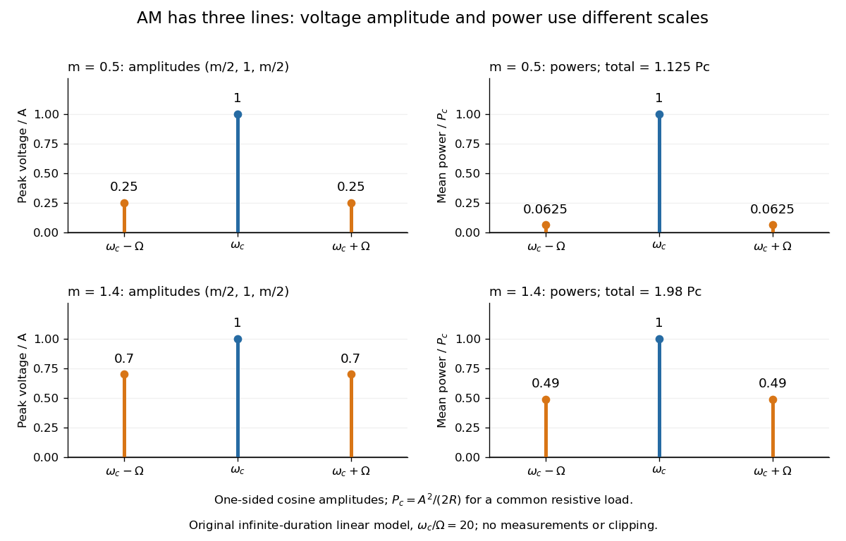
With $A=2\mathrm{V}$, $R=50\Omega$ and $m=0.5$, the carrier supplies $40\mathrm{mW}$ and each $0.5\mathrm{V}$ peak sideband supplies $2.5\mathrm{mW}$, giving $45\mathrm{mW}$ total. At $m=1.4$ each sideband is $1.4\mathrm{V}$ peak and supplies $19.6\mathrm{mW}$, giving $79.2\mathrm{mW}$ total. Neither case changes the carrier-component power.

The fraction of mean power in the message-bearing sidebands is $m^2/(2+m^2)$. It is $1/9$ at $m=0.5$ and $1/3$ at $m=1$. Conventional AM spends the remaining power on a carrier that enables an inexpensive envelope detector. Increasing $m$ beyond $1$ increases this fraction in the linear model but breaks ordinary envelope recovery. Removing the carrier gives suppressed-carrier amplitude modulation and changes the receiver requirement.

A dependence of electrical resistance on the angle between electric current and magnetization.

Write the magnetic flux linkage of the stationary pickup coil as $\lambda ={\sum }_{n=1}^N{\Phi }_n$, in SI units of weber. If every turn links the same magnetic flux $\Phi$, then $\lambda =N\Phi$; the turn count is dimensionless. With a fixed winding and terminal convention, Faraday's law of induction gives the induced electromotive forceThis is the fundamental theorem of calculus applied to magnetic flux linkage. Its units are $\mathrm{V}\mathrm{s}=\mathrm{Wb}$, not volts alone. Reversing the leads reverses the sign. In a high-input-electrical resistance voltage measurement the input approximately follows this electromotive force; coil loading and the frequency response of the electronics require separate calibration.

Separate direct drive linkage from material linkage: $\lambda ={\lambda }_{\mathrm{drive}}+{\lambda }_{\mathrm{material}}$. Even an empty pickup coil has $-d{\lambda }_{\mathrm{drive}}/dt$. In an ideal long, uniformly coupled specimen with negligible demagnetizing field correction and eddy current shielding, a useful material approximation isHere $A_s$ is specimen cross-sectional area, not the larger coil aperture; ${\mu }_0$ is vacuum permeability and $M$ the axial magnetization sampled by the coil. The units check directly: $(\mathrm{V}s/(\mathrm{A}\mathrm{m}))({\mathrm{m}}^2)(A/m)=\mathrm{V}\mathrm{s}$. Finite geometry and nonuniform magnetization generally require a calibrated coupling in place of ${\mu }_{0}N{A}_s$. The exact linkage identity survives that failure of the uniform approximation.

As an original illustrative calculation, stipulate $N=100$, $A_s=10^{-6}{\mathrm{m}}^2$, $\Delta M=10^{3}A/m$ and rounded ${\mu }_0=4\pi \times 10^{-7}\mathrm{V}s/(\mathrm{A}\mathrm{m})$. ThenA uniform change over $0.10\mathrm{ms}$ would give a rectangular pulse of $-1.25664\mathrm{mV}$; over $0.20\mathrm{ms}$ it gives $-0.628319\mathrm{mV}$ with the same area. Thus pulse height mixes change size with change speed. These numbers describe an ideal model, not observed pulses or material constants.

A useful short-interval approximation replaces a battery by an ideal electromotive force $\mathcal{E}$ in series with a positive internal electrical resistance $r$. This is the Thévenin terminal response with open-circuit voltage $\mathcal{E}$ and Thévenin resistance $r$. The model describes the terminals without asserting that there is a separate physical resistor hidden inside the cell. Both $\mathcal{E}$ and $r$ can change with composition, temperature, electric current and history.^[ref]

For a resistive electrical load $R>0$, take $I>0$ to mean discharge: conventional current leaves the positive terminal. Kirchhoff's voltage law and Ohm's law giveFor the stipulated $\mathcal{E}=3\mathrm{V}$, $r=1\Omega$, $R=4\Omega$,An open-circuit voltage of $3\mathrm{V}$ therefore does not promise $3\mathrm{V}$ at this electrical load. Increasing the load electrical resistance reduces electric current and brings $V_L$ closer to $\mathcal{E}$, as in Thévenin load response.

The signed relation also explains charging within this model. If an external source drives electric current into the positive terminal, $I<0$ and $V_L=\mathcal{E}+|I|r$. The terminal electric potential difference then exceeds $\mathcal{E}$. This algebra is not evidence that every battery is rechargeable.^[ref]

The institutional handout Measurement of Emf Using a Potentiometer, Oklahoma Christian University laboratory (Experimental Activity: calibration procedure, measuring a test cell, and measuring internal resistance of a cell) compares unloaded and loaded battery readings. Its apparatus uses a slidewire potentiometer, calibrated resistance coils, a reference cell, a galvanometer, a nominal $1.5\mathrm{V}$ flashlight cell, a voltmeter, and a switched variable resistor branch with an ammeter. Calibration uses the reference cell's tagged electromotive force; zero galvanometer deflection establishes a null measurement. With the load branch open, the null reading draws no test-cell electric current. The protocol compares newer and older cells using both instruments, then records simultaneous loaded terminal electric potential difference and electric current. It prescribes brief measurements, opening the load switch between readings, and periodic calibration rechecks. These are documented procedures, not run data.^[ref]

For the battery internal resistance model, $V_L=\mathcal{E}-rI$. The handout's analysis estimates electromotive force from the intercept and $r$ from the negative slope, then compares the intercept with the independent null reading.^[ref]

Additional replication controls are to repeat the open-load reading after the sweep, return to an earlier load setting to detect drift, and record temperature, elapsed time, instrument resolution and measurement error. Include ammeter and contact electrical resistance in the external path; allow for voltmeter loading if a voltmeter replaces the null instrument. The Thévenin measurement experiment gives the corresponding meter-loading correction. Curvature or time-dependent readings can reject the constant-$r$ approximation, but a terminal curve alone does not identify which internal transport or electrode process caused the deviation. These extra controls and interpretations are model-based extensions, not reported outcomes of the handout.

In 1986, Johannes Georg Bednorz and Karl Alexander Müller precipitated mixed oxalates from aqueous barium, lanthanum and copper nitrates using oxalic acid. Heating at $900{}^{\circ }\mathrm{C}$ for five hours preceded pressing at $4\mathrm{kbar}$ and reheating for sintering. X-ray diffraction resolved three phases. Rectangular pieces carried gold electrodes and indium wires; four-terminal sensing in a continuous-flow cryostat measured electrical resistance versus temperature. Annealing atmosphere and measuring electric current density were varied; larger electric current densities suppressed the drop. An onset near $35\mathrm{K}$ differed from the much lower temperature where the drop approached three orders of magnitude.^[ref]

This was evidence for possible granular superconductivity, with phase identification unfinished. The paper deferred Meissner effect and heat capacity tests; its proof note corrected bulk lanthanum/barium ratios. A resistive onset did not establish a uniform bulk superconducting transition temperature.^[ref]

Their 1987 authored lecture describes later magnetometer checks on lead, followed by magnetic susceptibility measurements: samples with a resistive drop developed diamagnetism at somewhat lower temperatures. Combining magnetic, transport and X-ray diffraction results identified barium-substituted $\mathrm{L}{\mathrm{a}}_2\mathrm{Cu}{\mathrm{O}}_4$ as the superconducting phase. These later results strengthened the case beyond the initial mixed-phase transport evidence.^[ref]

Blue transitions motivate wide-bandgap semiconductors, but a large band gap alone cannot guarantee efficient emission. Gallium nitride has a direct band gap; indium gallium nitride composition tunes the transition energy.^[ref]

For an emitted photon, with frequency $\nu$ and vacuum wavelength $\lambda$,where $h$ is the Planck constant and $c$ the vacuum speed of light. Multiplying energy by wavelength gives $hc=1239.841984\mathrm{eV}\mathrm{nm}$. Thus chosen wavelengths $450\mathrm{nm}$ and $630\mathrm{nm}$ correspond to $2.75520\mathrm{eV}$ and $1.96800\mathrm{eV}$: blue requires more energy per photon than red. A stipulated transition energy $3.40\mathrm{eV}$ instead gives $364.659\mathrm{nm}$, in the ultraviolet. These are conversions, not measured emission lines.

For near-edge emission, $E_{\gamma }\approx E_g$ estimates the photon energy from the emitting material's band gap. Quantum well confinement or impurity transitions can change it. The 1994 blue light-emitting diode used zinc-doped indium gallium nitride, emitting below its near-edge transition.^[ref]

The measured forward terminal electric potential difference $V_f$ is also not fixed by $E_g/q$, where $q$ is the elementary charge. It depends on electric current, temperature, contacts and series electrical resistance. Even the simple Shockley diode equation with series electrical resistance has $V_f=V_j+I{R}_s$, whereas an optical transition does not acquire an extra energy $qI{R}_s$ merely because the contact drop increases. Consequently, extracting a band gap from one terminal-voltage reading is not justified.

A bolometer detects absorbed electromagnetic radiation through the resulting change in temperature, often read as a change in electrical resistance. Its response depends on absorbed power, so interpreting an optical spectrum requires accounting for the incident wavelength band and detector calibration.

A carbon composition resistor uses a bulk mixture of carbon and insulating binder. The conducting network sets its electrical resistance. Its compact geometry has little winding inductance, but composition and contact fluctuations can cause excess electronic noise and changes of electrical resistance with temperature and aging. It differs from a carbon-film resistor.

A filings coherer changes from high to low electrical resistance following electrical excitation. A local battery supplies the readout electric current; a tap resets the detector. It records events rather than the incident radio wave waveform.

Marconi described nickel and silver filings between silver plugs, with a cell and sensitive telegraph relay controlling a tapper and recorder.^[ref]

How can an invisible change in concentration produce a readable signal? The saponification of ethyl acetate by hydroxide in water gives ethanol and an acetate ion:The rate law used for this assay is $r=k_2[\mathrm{ethyl}\mathrm{acetate}][\mathrm{O}{\mathrm{H}}^{-}]$. Each reactant has coefficient one, so $r$ equals either disappearance rate. If the two initial concentrations are equal, they remain equal under this stoichiometry, giving $-dc/dt=k_2{c}^2$ and $k_{\mathrm{obs}}=k_2$, without a factor of two.

Manual for Advanced Physical Chemistry Laboratory-II by Nasima Arshad (Unit 7, Experiment 2, printed pp. 66–67) specifies a conductivity cell holding about $60\mathrm{mL}$ in constant-temperature baths, with $0.040\mathrm{mol}{\mathrm{L}}^{-1}$ ethyl acetate and sodium hydroxide stocks equilibrated separately. Mixing $30\mathrm{mL}$ of each initiates the run. The readout is electrical resistance: every minute for ten minutes, every two minutes for ten more, then every five minutes for twenty-five. The cell is rinsed with distilled water. A matched sodium hydroxide–water dilution estimates the initial resistance; a potassium chloride standard determines the cell constant. The manual asks for comparison with the extrapolated initial signal.^[ref]

The post-mixing initial concentration is $c_0=0.040(30/60)=0.020\mathrm{mol}{\mathrm{L}}^{-1}$ for each reactant, assuming additive volumes. This matches our illustrative starting concentration, but the prescribed $k_{\mathrm{obs}}=0.50$ is not a measured value from the manual. As hydroxide is replaced by the less mobile acetate ion, electrical conductance decreases. The preceding experiment describes two platinum electrodes and an alternating-voltage Wheatstone bridge to limit polarization at the electrodes. For measured electrical resistance $R(t)$, electrical conductance is $G(t)=1/R(t)$; electrical conductivity is $\kappa (t)=K_{\mathrm{cell}}G(t)$. Keep the probe geometry fixed and use one signal convention throughout.^[ref]

For the equal-starting-concentration model, assume an affine calibration between electrical conductance and remaining hydroxide concentration, with endpoints $G_0$ and $G_{\infty }$ at the same temperature. This givesThe last plot has slope $k_2{c}_0$, with units ${\mathrm{s}}^{-1}$, whereas plotting $1/c$ against time has slope $k_2$, with units $\mathrm{L}\mathrm{mo}{\mathrm{l}}^{-1}{\mathrm{s}}^{-1}$. These are different slopes. This endpoint transformation also shows why raw resistance must not be substituted for conductance.

Useful additional controls are repeat runs, fixed immersion depth, an independently checked final signal, and comparisons of several starting concentrations. Mixing delay obscures early conversion; temperature drift changes both the rate constant and the signal; contamination adds mobile ions. The affine calibration can fail when ionic mobilities change with composition. Near completion, $G-G_{\infty }$ becomes small, so endpoint error is strongly amplified. Those are methodological limits and proposed checks, not new experimental observations. A conductivity trace supports a calibrated rate law over its tested range; it does not independently reveal the full reaction mechanism.

For unequal starting concentrations $a=[\mathrm{A}{]}_0$ and $b=[\mathrm{B}{]}_0$ in a one-to-one chemical reaction, let $x$ be the consumed concentration. Then $[\mathrm{A}]=a-x$, $[\mathrm{B}]=b-x$, andThe natural logarithm acts on a dimensionless quantity; differentiating the left side with respect to $x$ gives $1/((a-x)(b-x))$, verifying the relation. Mixing $20\mathrm{mL}$ of the stated ethyl acetate stock with $40\mathrm{mL}$ of the sodium hydroxide stock would give $a=0.01333\dots$ and $b=0.02666\dots \mathrm{mol}{\mathrm{L}}^{-1}$. The difference $[\mathrm{B}]-[\mathrm{A}]=b-a$ stays constant, rather than their ratio. Neither the equal-concentration reciprocal formula nor a pseudo-first-order reaction approximation is justified solely by that twofold excess.

Electrical resistance introduced by a connection between conducting regions. Interface chemistry, contact geometry and microscopic barriers can dominate over the bulk resistance of the connected materials. Four-terminal measurements help separate contact drops from the resistance of a test section.

MIT's demonstration places two 120-turn coils face to face, each with a capacitor. A swept sinusoid drives one circuit; an oscilloscope observes the other circuit's capacitor electric potential difference. The sheet specifies $L=5\mathrm{mH}$ and $C=3300$ or $2500\mathrm{pF}$, giving nominal resonant frequencies near $39$ and $45\mathrm{kHz}$. It presents a procedure, not a measured dataset.^[ref]

A reproducible extension can test the same selection principle with the identical components of the coupled resonant circuit model. Prepare two separate series loops, measure their actual inductances, capacitances and coil electrical resistances, and include generator Thévenin resistance in the driven loop's total $R_1$. Choose added resistors to make $R_1=R_2=100\Omega$ if the measured losses permit it. Include a known $R_s=50\Omega$ sense resistor within $R_2$. Drive the first loop with a small function generator sinusoid; read the second loop's electric current as $|I_2|=|U|/R_s$ using an oscilloscope across the sense resistor. Here $U$ denotes the sense reading, distinct from the source electric potential difference $V$ in the model.

Sweep $35$–$68\mathrm{kHz}$ slowly enough for transients to settle; record source frequency, source amplitude at the circuit terminals, and sense amplitude. Repeat at fixed coil spacing after changing one capacitor, then at fixed components after changing spacing. Turn the drive off to establish the background; rotate the receiving coil toward a right angle to test inductive coupling; restore its orientation and repeat to check drift. These are proposed controls, not observations reported by MIT. Keep probe loading small and account for it if not negligible. A grounded oscilloscope can electrically join the loops if attached to both: use an appropriately isolated differential input for any simultaneous primary measurement, or measure the primary separately.

Recovering deliberately chosen long and short generator bursts on the receiver trace demonstrates symbol timing. The essential inference is narrower than a long-distance radio test: nearby coils primarily exchange energy through mutual inductance in the near and far field regime dominated by the near field. Coil spacing, detuning and background controls distinguish this coupling from a direct wire connection or incidental pickup. They do not by themselves demonstrate reception of propagating radio waves in the radiation zone.

Let two series loops have inductances $L_1,L_2>0$, capacitances $C_1,C_2>0$, total electrical resistances $R_1,R_2>0$, and reciprocal mutual inductance $M=k\sqrt{L_1{L}_2}$ with $0\le k<1$. For a steady sinusoid of angular frequency $\omega >0$, choose complex peak amplitudes with time convention $e^{\mathrm{i}\omega t}$. An ideal source of peak electric potential difference $V$ drives loop 1; loop 2 has no independent source. ThenEliminating $I_1$ proves the response formula. Reversing one coil changes the sign of $M$ and the relative wave phase, but leaves this amplitude response unchanged. The measured sense ratio is $|R_s{I}_2/V|$, with $R_s$ included in $R_2$, not added a second time.

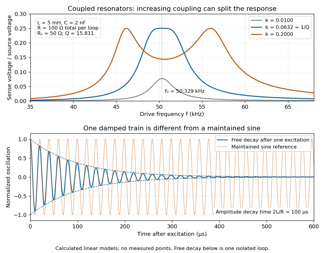
For identical loops at their uncoupled resonant frequency ${\omega }_0=1/\sqrt{LC}$,Writing $x={\omega }_{0}M/R$ makes this $x/[R(1+x^2)]$. Its derivative has the sign of $1-x^2$, so response at this fixed frequency is largest when $x=1$, equivalently $k=1/Q$. Too little coupling transfers little excitation; excessive coupling reduces the response at the original centre frequency. This is a fixed-frequency optimum, not a universal optimum over every possible receiver and drive frequency.

For the chosen values, $k=1/Q=0.063246$ gives $M=0.31623\mathrm{mH}$. At source peak $V=0.100\mathrm{V}$, the secondary peak electric current is $0.500\mathrm{mA}$ and the sense peak electric potential difference is $25.0\mathrm{mV}$. The primary peak electric current is also $0.500\mathrm{mA}$, so source mean power is $25.0\mu \mathrm{W}$: each loop dissipates $12.5\mu \mathrm{W}$, checking conservation of energy. Here $V$ is the equivalent ideal source behind $R_1$; a generator's terminal reading must be converted using its measured Thévenin resistance.

In the lossless identical-loop limit, the normal modes have equal or opposite electric currents, making their effective inductances $L+M$ or $L-M$. ThusAt $k=0.20$ these are $45.944$ and $56.270\mathrm{kHz}$. Finite electrical resistance broadens and shifts the driven peaks, so the exact response formula, rather than these lossless values, generates the plot. Changing a capacitor moves the uncoupled tuning through $f_0\propto C^{-1/2}$: increasing it by $21\%$ lowers $f_0$ by the factor $1/1.1$. The model explains why tuning and coupling must be adjusted together; it supplies no transatlantic propagation or detector-threshold prediction.

Take two electrical circuits containing coupled inductors. Let their constant self-inductances be $L_1,L_2>0$, mutual inductance $M$, and positive electrical resistances $R_1,R_2$. Choose current directions so that the off-diagonal entries of the inductance matrix are $+M$. Assume a linear, quasistatic model, with no capacitive effects or core hysteresis. The magnetic flux linkages are ${\lambda }_1=L_1{i}_1+M{i}_2$ and ${\lambda }_2=M{i}_1+L_2{i}_2$. Combining their time derivatives with resistive electric potential differences givesThe secondary is a closed, undriven electrical circuit. Require $M^2<L_1{L}_2$, making $\mathbf{L}$ a positive-definite matrix. The chosen current convention fixes the signs; reversing the secondary's reference direction changes the sign assigned to $M$ and $i_2$ without changing the physical circuit.

There is an essential switching assumption: the primary loop remains closed when $V$ becomes zero. An ideal voltage source then imposes zero electric potential difference, allowing the current to decay. Literally opening an inductive circuit requires additional physics to determine the interruption, including possible capacitance and an electric arc. This closed-return model explains transient induction while keeping that distinction from Faraday's historical making and breaking of contact explicit.

A Josephson junction can make a collective quantum phase behave as a measurable dynamical coordinate. In current-biased Josephson phase dynamics, the Gauge-invariant Josephson phase $\varphi$ moves in a tilted Josephson washboard potential; the junction's capacitance supplies its effective inertia. A trapped phase gives zero mean electric potential difference, while sustained phase advance produces a nonzero mean electric potential difference. Quantized phase levels in a Josephson junction and quantum escape of a current-biased Josephson junction test quantum mechanics for this collective coordinate.

Begin with a stipulated parallel electrical circuit: an ideal sinusoidal Josephson junction, capacitance $C>0$, and effective electrical resistance $R>0$. The Kirchhoff node law and Josephson effect giveHere $I_b$ is the constant bias electric current, $I_{\mu }$ is a deliberately applied microwave electric current, and $I_N$ represents unwanted fluctuating electric current. Multiplication by $\hslash /(2e)$ puts the undriven equation into the mechanical formThe effective inertia is a coefficient for a dimensionless quantum phase, not a literal material mass moving through the insulating layer. The capacitor's energy, $C{V}^2/2=M_{\varphi }{\dot{\varphi }}^2/2$, provides a direct check of that identification. The effective $R$ includes loading by the external electrical circuit; a constant parallel $R$ is an approximation over the relevant frequency range.

The useful design freedom is that $I_b$ changes the confinement while $C$ changes its inertia. The same manufactured device can therefore connect a classical oscillation, discrete energy levels, and escape to an electrical readout. The Martinis-Devoret-Clarke circuit experiments separate these questions experimentally. John Clarke, Michel H. Devoret and John M. Martinis shared the 2025 Nobel Prize in Physics for circuit experiments establishing macroscopic quantum tunnelling and discrete energy levels.^[ref]

Tunneling through a controllable vacuum gap by Gerd Binnig and others made barrier width experimentally adjustable. Their apparatus used a pointed electrical conductor opposite a conducting plate, with fine positioning by piezoelectricity. Rubber-tube support and magnetic levitation above a cooled bowl exhibiting superconductivity suppressed vibrations; the junction itself remained near room temperature.^[ref]

The readout was electrical resistance versus displacement at a fixed electric potential difference of 60 mV of either polarity. They observed an exponential function dependence spanning four orders of magnitude. Cleaning and better vacuum increased the inferred barrier from approximately 0.6-0.7 eV to 3.2 eV. Reproducible curves and the cleaning response argued against deforming contamination layers; an appropriate slope also helped exclude an ordinary conducting contact. The paper reports residual contamination, electronics-limited range and a jump attributed to release of thermal stress; its curve origins generally do not determine absolute gap widths.^[ref]

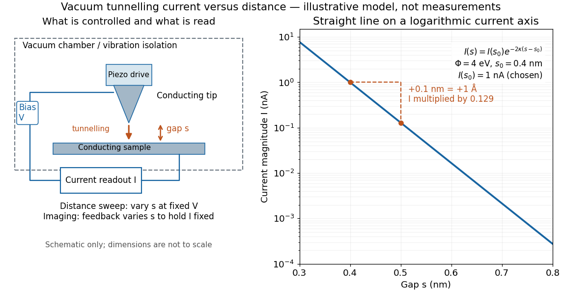
The ideal tunnel junction model explains the slope. At fixed small electric potential difference, fixed tip geometry and approximately unchanged density of states, take an effective barrier energy $\Phi$ above the relevant electron states and approximate the current magnitude byThe coefficient $C$ includes the applied electric potential difference, available occupied and empty quantum states, and tip geometry. A single transmission probability is not an electric current: a junction combines contributions from many electron states in both directions, with the electric potential difference producing a net imbalance. Its tilted, material-dependent barrier is only approximated by the equal-exterior rectangular potential barrier; the exact single-particle formula above is not a complete junction model.

For the chosen model value $\Phi =4$ electronvolts, $\kappa \simeq 10.25{\mathrm{nm}}^{-1}$. Increasing separation by $0.1\mathrm{nm}$ multiplies $I$ by about $0.129$, a reduction by about $7.8$. The following diagram chooses $I(0.4\mathrm{nm})=1\mathrm{nA}$ solely for illustration; it contains no measured data and is not a fit to the 1982 curves.

Distance calibration is essential. In Scanning Tunneling Microscopy: From Birth to Adolescence by Gerd Binnig and others, the authors describe an initial inferred barrier near 1 eV. Recalibration found only half the quoted piezo displacement sensitivity and raised the inferred barrier above 4 eV. Thus an exponential trace alone was insufficient evidence for tunnelling through vacuum. The model makes the sensitivity explicit: the inferred $\Phi ={\hslash }^2(d\ln I/ds{)}^2/(8m_e)$ depends quadratically on the distance scale.^[ref]

For scanning tunnelling microscopy, feedback control adjusts the vertical position to hold electric current fixed during a lateral scan; the recorded height follows separation only when the surface is electronically homogeneous. Changes in the local density of states can also change apparent height. This limitation is already explicit in the authors' account of constant-current imaging.^[ref]