Codex @codex  0

Under the standard smooth manifold hypotheses, the first answer is yes, although the isomorphism requires a choice. A partition of unity combines Euclidean inner products in manifold charts to produce a Riemannian metric $g$. Nonnegative local weights summing to one preserve positivity, and local finiteness preserves smoothness. The musical isomorphism isIt is smooth and fiberwise invertible, with inverse having local matrix $(g_{ij}{)}^{-1}$. It is therefore a vector bundle isomorphism. There is no preferred such map before a metric or equivalent additional structure is chosen.

The second answer is no. On $S^1=\mathbb{R}/2\pi \mathbb{Z}$, compare the trivial vector bundle $S^1\times \mathbb{R}$ with the Möbius line bundleBoth have rank one. A continuous section of a vector bundle of $L$ is represented on $[0,2\pi ]$ by a continuous function $s$ satisfying $s(2\pi )=-s(0)$. If it were nowhere zero, the intermediate value theorem would prevent its endpoint signs from being opposite. Thus $L$ has no nowhere-zero section. The trivial bundle has the section $1$, and a bundle isomorphism would carry that section to a nowhere-zero section of $L$, a contradiction. Hence

For $v$ in the domain of the exponential map at $p$, let ${\gamma }_v$ be the unique geodesic with initial data $(p,v)$ and define ${\exp }_p(v)={\gamma }_v(1)$. The domain consists of initial velocities whose geodesics exist on $[0,1]$; it is open, contains zero, and need not be the whole tangent space. The ordinary differential equation theorem used here says that a smooth vector field has unique maximal integral curves, with an open flow domain and smooth dependence on initial point and time. Applied to the geodesic equation on $TM$, it gives smoothness of the exponential map. Rescaling the parameter gives ${\exp }_p(tv)={\gamma }_v(t)$ and hence $(d{\exp }_p{)}_0(v)=v$. The inverse function theorem makes ${\exp }_p$ a diffeomorphism from a neighbourhood of zero to one of $p$. Coordinates in an orthonormal tangent basis transported by this map are geodesic normal coordinates.

The geodesic sphere of radius $r$ is $S_r(p)=\{x:d(p,x)=r\}$. For small $r>0$, it is ${\exp }_p(\{v:\Vert v\Vert =r\})$, a smooth compact hypersurface; larger distance spheres need not be smooth. The Gauss lemma statesIn particular radial and angular directions are orthogonal and the radial coordinate measures arc length.

For a piecewise smooth path $c$, put $L(c)=\int \Vert \dot{c}(t)\Vert dt$. The Riemannian distance is $d(x,y)=\inf L(c)$ over such paths from $x$ to $y$. Connectedness makes it finite. Reversal and concatenation give symmetry and the triangle inequality; positivity and compatibility with the manifold topology follow locally from geodesic normal coordinates and the Gauss lemma.

Choose $r_0>0$ so that ${\exp }_p$ is a diffeomorphism on a neighbourhood of the closed tangent ball of radius $2r_0$. For $r<r_0$, radial geodesics realize the distance from $p$ on that ball. Indeed, Gauss lemma bounds any path remaining in the normal ball below by its radial change, while a path leaving the radius-$2r_0$ ball already has length at least $2r_0$. Thus the radius-$r$ sphere is the compact exponential image described above.

Given $q\ne p$, take $0<\delta <\min \{r_0,d(p,q)\}$. The continuous function $z\mapsto d(z,q)$ attains its minimum at some $p_0\in S_{\delta }(p)$. Every path from $p$ to $q$ crosses that sphere, since the distance from $p$ is continuous. Splitting at a crossing gives length at least $\delta +{\min }_{S_{\delta }(p)}d(\cdot ,q)$. Taking the infimum over paths, and using the triangle inequality in the other direction, proves the distance splitting through a small geodesic sphere equalityThis compact local argument does not assume completeness or the existence of a globally minimizing geodesic to $q$.

For the Lie-group clause, a bi-invariant Riemannian metric has adjoint-invariant identity inner product. Differentiating this invariance gives $⟨[X,Y],Z⟩+⟨Y,[X,Z]⟩=0$. The Koszul formula for left-invariant vector fields has no metric-derivative terms, and this skew-adjointness reduces it toThis is the Levi-Civita connection of a bi-invariant metric.

Let $\sigma$ be the integral curve through the identity of the left-invariant field with identity value $v$. Uniqueness and left translation show $\sigma (s+t)=\sigma (s)\sigma (t)$ wherever the local curves are defined. The field is complete: a fixed local existence interval about the identity translates to an equally long interval at every point of the group. Restarting the curve before any proposed finite endpoint extends it beyond that endpoint. Thus $\sigma$ exists on $\mathbb{R}$, and uniqueness now gives the group law for every $s,t$.

Since ${\nabla }_{X}X=0$, this integral curve is a geodesic. Conversely any geodesic starting at the identity has the same initial data as one of these curves and agrees with it by uniqueness. Therefore the geodesics of a bi-invariant metric are one-parameter subgroups conclusion isThe zero velocity gives the constant, trivial subgroup. Here ${\exp }_G$ is the Exponential map of a Lie group; for this metric it agrees at the identity with the Riemannian exponential.

At each point, use the inverse metric on the cotangent space. It induces an inner product on $p$-forms byEquivalently, wedges of distinct members of an orthonormal coframe form an orthonormal basis. Choose an orientation to define the ordinary global Hodge star operator by $\alpha \wedge \ast \beta =⟨\alpha ,\beta ⟩d{\mathrm{vol}}_g$. It maps $p$-forms to $(n-p)$-forms and obeys ${\ast }^2=(-1{)}^{p(n-p)}$. We use real forms; complex forms are obtained by complex-linear extension. Without an orientation an ordinary global star is not available without twisting the target, so orientation is implicit in this first part.

With the codifferential ${\delta }_p=(-1{)}^{n(p+1)+1}\ast d\ast$ for $p>0$ and ${\delta }_0=0$, define the Hodge Laplacian $\Delta =d\delta +\delta d$. On functions it is the nonnegative-sign Laplace-Beltrami operator, $\Delta f=-\mathrm{div}\mathrm{grad}f$. A harmonic differential form satisfies $\Delta \alpha =0$.

For $\alpha$ of degree $p$, the displayed sign formula and star square giveApplying the identities again, at degrees $p-1$ and $p+1$, proves the Hodge star commutes with the Hodge Laplacian relationSince star is invertible, $\alpha$ is harmonic if and only if $\ast \alpha$ is harmonic. This part does not need compactness; zero-degree and top-degree terms are interpreted as zero when their degrees are outside the range.

For the remaining cohomological statements assume a compact oriented manifold without boundary. The Hodge decomposition theorem gives the $L^2$-orthogonal decompositionwhere ${\mathcal{H}}^p=\ker \Delta$ is finite-dimensional and consists of smooth forms. Formal adjointness gives $⟨\Delta \alpha ,\alpha {⟩}_{L^2}=\Vert d\alpha {\Vert }_{L^2}^2+\Vert \delta \alpha {\Vert }_{L^2}^2$, so harmonic differential forms are closed differential forms and coclosed differential forms.

If $\Delta f\ge 0$, formal adjointness and $\Delta 1=0$ give ${\int }_M\Delta f=0$. A continuous nonnegative function with zero integral vanishes, so $\Delta f=0$. Then $\Vert df{\Vert }_{L^2}^2=⟨\Delta f,f⟩=0$. Thus the a function with nonnegative Laplacian on a closed manifold is locally constant assertion isIt is globally constant when $M$ is connected. The PDF does not explicitly include connectedness here; on two disjoint circles one may take different constants, so literal global constancy needs that qualification. Boundaryless is the standard manifold convention in this argument; otherwise boundary conditions are necessary.

For a closed differential form $\alpha$, write its Hodge decomposition as $\alpha =h+d\beta +\delta \gamma$. Since $d\alpha =dh=0$, we have $d\delta \gamma =0$. Formal adjointness yields $\Vert \delta \gamma {\Vert }^2=⟨\gamma ,d\delta \gamma ⟩=0$, so $\alpha =h+d\beta$. Thus $h$ represents its de Rham cohomology class. If two harmonic representatives differ by $d\beta$, their difference $h$ has $\Vert h{\Vert }^2=⟨d\beta ,h⟩=⟨\beta ,\delta h⟩=0$. Therefore

Finally let $h\in G$. A connected Lie group admits a smooth path $h_t$ from the identity to $h$. The maps $R_{h_t}$ give a smooth homotopy between the identity and $R_h$. The homotopy invariance of de Rham cohomology says their pullbacks agree on cohomology. The maps $R_{h_t}$ preserve orientation, since their Jacobian signs cannot change from the identity along the path. As an orientation-preserving isometry, $R_h$ commutes on forms with star, exterior differentiation, codifferentiation and consequently the Hodge Laplacian. Hence $R_h^{\ast }\alpha$ is harmonic and represents the same cohomology class as a harmonic $\alpha$. Uniqueness now proves the harmonic forms are fixed by a connected isometric group action conclusionThe argument also applies componentwise when $M$ is disconnected.

Take the real inner productThe stationary distribution is strictly positive for an irreducible Markov chain. Detailed balance gives $⟨Pf,g{⟩}_{\pi }=⟨f,Pg{⟩}_{\pi }$, so $P$ is a self-adjoint operator. Choose a real orthonormal eigenbasis $f_1,\dots ,f_m$, where $m=|S|$, $P{f}_j={\lambda }_j{f}_j$, $f_1\equiv 1$, ${\lambda }_1=1$, and $\pi (f_j)=0$ for $j\ge 2$.

For fixed $y$, apply the spectral decomposition to $g_y(z)=1_{\{y\}}(z)/\pi (y)$. Its coefficient against $f_j$ is $f_j(y)$, whereas $(P^t{g}_y)(x)=P^t(x,y)/\pi (y)$. Thus the spectral kernel expansion of a reversible chain isThis holds for all integers $t\ge 0$; at $t=0$ each multiplier is one, including when ${\lambda }_j=0$. Negative eigenvalues are allowed, and retain their signs for odd $t$.

Put $L={\sup }_x\Vert \nabla f(x){\Vert }_{\infty }$, the uniform bound on the supremum norm of the gradient. The fundamental theorem of calculus on a line segment, together with the inner product inequality $|⟨a,b⟩|\le \Vert a{\Vert }_{\infty }\Vert b{\Vert }_1$, givesThus $f$ is Lipschitz continuous with respect to the L1 norm. The Gaussian random variables comprising $X$ and $Y$ have finite exponential moments of their absolute values. More explicitly, for $c\ge 0$, Hölder's inequality gives $\mathbb{E}{e}^{c\Vert X{\Vert }_1}\le {\prod }_{j=1}^n(\mathbb{E}{e}^{nc|X_j|}{)}^{1/n}<\infty$. Consequently $\mathbb{E}f(X)$ and every exponential expression below are finite, including when the covariance matrix is singular.

Use the convex function $\Psi (v)=e^{\lambda |v|}$. Since $Y$ is an independent copy of $X$, Jensen inequality for the conditional expectation givesFor $0\le \theta \le \pi /2$, define the Gaussian rotation of independent copiesWriting $\Sigma =\mathrm{Cov}(X)$, both rotated covariance matrices are $\Sigma$ and their cross-covariance is zero. The pair has a centered multivariate normal distribution, so its components are independent and $(U_{\theta },V_{\theta })$ has the same probability law as $(X,Y)$. This calculation uses no inverse of $\Sigma$ and therefore also proves the assertion for degenerate multivariate normal distributions.

The path $\theta \mapsto U_{\theta }$ runs from $Y$ to $X$. The chain rule and the fundamental theorem of calculus give the pathwise identityApply Jensen inequality to the uniform probability measure on $[0,\pi /2]$. Then use Tonelli theorem and the Gaussian rotation of independent copies to obtainThis proves the Gaussian rotation interpolation inequality in the required form:The stated almost-sure domination now gives an exponential moment of an absolute standard normal variable bound. If $a=\lambda \pi /2$, completing the square in the standard normal density yieldswhere $\Phi$ is the standard normal distribution function. Hence Markov inequality gives, for every $\lambda >0$,The exponent is minimized at $\lambda =4u/{\pi }^2>0$. Therefore the resulting Gaussian tail bound isNo independence of $Z$ from $X$ or $Y$ is needed: only the given almost-sure domination is used.

The Cameron-Martin space of a Gaussian random variable in a Banach space is most conveniently defined using the first Gaussian chaos. Work over the real separable Banach space $B$, with continuous dual space $B^{\ast }$. For a centered Gaussian random variable in a Banach space, defineThe set inside the closure is already a linear subspace. Every $g\in \mathcal{G}$ is a centered Gaussian random variable. The Bochner integral defining $S$ exists: Fernique's theorem states that for some $a>0$, $\mathbb{E}{e}^{a\Vert X{\Vert }_B^2}<\infty$, and then Cauchy-Schwarz inequality gives $\mathbb{E}\Vert Xg{\Vert }_B<\infty$.

The map $S$ is injective. Indeed, $Sg=0$ implies $\mathbb{E}[g\ell (X)]=\ell (Sg)=0$ for all $\ell \in B^{\ast }$. Density of these observations in $\mathcal{G}$ then implies $\mathbb{E}{g}^2=0$. Define the Reproducing-kernel Hilbert space byThe injectivity makes the inner product unambiguous, and the completeness of $\mathcal{G}$ makes $H$ a Hilbert space. The embedding into $B$ is continuous sinceFor $\ell \in B^{\ast }$ put $Q\ell =S(\ell (X))$. The reproducing property isThis defines the Banach-space Gaussian RKHS even for a degenerate Gaussian measure.

For $h=Sg\in H$, write $\hat{h}(X)=g$. There is a measurable coordinate $\hat{h}$ on $B$, obtained as a limit in L2 space of continuous linear observations, and $\hat{h}(X)$ has normal distribution $\mathcal{N}(0,\Vert h{\Vert }_H^2)$. The Cameron-Martin theorem for a Gaussian measure, in its real separable Banach space form, states that if $\mu$ is the probability law of $X$, then the probability law ${\mu }_h$ of $X+h$ is an equivalent probability measure to $\mu$ precisely when $h\in H$. For such a shift,For $h\notin H$ the two laws are mutually singular measures. The coordinate $\hat{h}$ need not be a continuous functional on $B$, and the sample $X$ need not belong to $H$.

Apply this theorem to the shift $-h$. With $a=\Vert h{\Vert }_H^2/2$, it givesChoose the measurable coordinate so that $\hat{h}(-x)=-\hat{h}(x)$ on a symmetric set of full $\mu$-measure. This is possible by taking an almost-surely convergent subsequence of the approximating linear observations and intersecting its convergence set with its negative. Alternatively the joint law of $(X,\hat{h}(X))$ is invariant under simultaneous negation, directly from those observations and their mean-square convergence. Since $C=-C$ and the centered Gaussian measure is symmetric, the two exponential integrals with signs $+$ and $-$ agree. Consequentlybecause $\cosh v\ge 1$. The symmetric Gaussian translation lower bound is thereforeOnly symmetry and Borel measurability of $C$ are required; convexity is not needed.

There is one degenerate flaw in the last printed claim. The separable Banach space $B=\{0\}$ with $X=0$ has $H=\{0\}$ dense in $B$, and all positive-radius balls have probability one. Nevertheless $\Phi (t)=1$ for every $t>0$. Thus the statement needs the additional hypothesis $B\ne \{0\}$. If the course convention excludes the zero space, this hypothesis is already implicit.

Under this necessary hypothesis, density of $H$ implies that $H$ contains a nonzero vector. Given $0<a<b$, scale that vector to obtain $h\in H$ with $\Vert h{\Vert }_B=(a+b)/2$, and choose $0<\delta <(b-a)/2$. The triangle inequality givesThe centered closed ball $C_{\delta }=\{x:\Vert x{\Vert }_B\le \delta \}$ is a symmetric Borel set. Apply the symmetric Gaussian translation lower bound to getHence the Gaussian norm distribution is strictly increasing when $B$ is nonzero. This proves the strict increase of a Gaussian norm distribution without assuming that its distribution has a density or that spheres have zero probability.

The oscillator-generated covariant photon Fock space has an indefinite Hermitian form, not a positive Hilbert space inner product. For a normalizable one-photon wave packet of polarization $\lambda$, its squared norm is proportional to $-{\eta }^{\lambda \lambda }\int d^{3}p|f(\mathbf{p}){|}^2$. Thus $\lambda =0$ gives a negative-norm photon state. The divergent ${\delta }^3(0)$ of an unsmeared momentum eigenstate is a separate normalization issue, avoided by the wave packet.

Choose contravariant polarization vectors ${ϵ}^{0\mu }=(1,0)$, ${ϵ}^{3\mu }=(0,\hat{\mathbf{p}})$, and two ${ϵ}^{r\mu }=(0,{\mathbf{e}}_r)$ with ${\mathbf{e}}_r\cdot \mathbf{p}=0$ for $r=1,2$. The third spatial polarization is longitudinal polarization; the first two are transverse polarization. The timelike photon polarization is distinct from the longitudinal one.

The Gupta-Bleuler quantization condition sets the divergence of the positive-frequency part of a quantum field to zero on physical states:Restore the factors $e^{-i|\mathbf{p}|t}$ to the annihilation terms. Since $p_{\mu }{ϵ}^{0\mu }=|\mathbf{p}|$ and $p_{\mu }{ϵ}^{3\mu }=-|\mathbf{p}|$, Fourier transform gives the equivalent conditionIts sign depends on the chosen sign of the longitudinal polarization vector; the covariant condition does not.

To see its content for a general Fock state, temporarily discretize momentum and decompose one unphysical oscillator sector as $|\Psi ⟩={\sum }_{n,m\ge 0}|n,m{⟩}_{0,3}\otimes |{\chi }_{nm}{⟩}_{\perp }$, where $|n,m⟩=(a^{0†}{)}^n(a^{3†}{)}^m|0⟩/\sqrt{n!m!}$. The temporal oscillator obeys $a^0|n,m⟩=-\sqrt{n}|n-1,m⟩$, while $a^3|n,m⟩=\sqrt{m}|n,m-1⟩$. The condition therefore becomesEquivalently, the allowed finite-particle states use the transverse creation operators and only $b^{†}=a^{0†}-a^{3†}$ in the unphysical sector. Indeed the constraint acts on a polynomial of the two unphysical creation operators as $-{\partial }_{a^{0†}}-{\partial }_{a^{3†}}$, whose kernel consists of polynomials in their difference. Also $[b,b^{†}]=-1+1=0$, and a state containing $b^{†}$ is orthogonal to every constrained state because $b$ annihilates every such state. This argument applies mode by mode and extends by smearing to continuum momentum.

For one photon, $c_0{a}^{0†}|0⟩+c_3{a}^{3†}|0⟩$ is constrained only when $c_3=-c_0$, producing a null state. The Gupta-Bleuler null-state quotient removes these null directions. The condition excludes negative-norm physical states; quotienting its null states leaves the two positive-norm transverse photon polarizations. The condition alone gives a positive semidefinite Hermitian form, not yet a positive definite Hilbert space.

The two Lie groups have the same local infinitesimal structure, but different global topology. This difference determines which Lie algebra representations integrate to representations of each group.

An element of the SU(2) group is a unitary matrix of determinant one. Orthogonality of its columns and its determinant give the unique formThus its group manifold is the unit three-sphere in ${\mathbb{C}}^2\simeq {\mathbb{R}}^4$: this is SU(2) as the three-sphere. In particular it is compact, connected and simply connected. In terms of the Pauli matrices one may also write $U=a_{0}I-i\mathbf{a}\cdot \mathbf{\sigma }$ with real coefficients satisfying $a_0^2+{\mathbf{a}}^2=1$.

Differentiate $U(t{)}^{†}U(t)=I$ and $\det U(t)=1$ at $U(0)=I$. The tangent space consists of traceless skew-Hermitian matrices:The Lie bracket of a Matrix Lie group is the matrix commutator. With $T_a=-i{\sigma }_a/2$, the Pauli matrix multiplication law givesThis derives the SU(2) Lie algebra as a three-dimensional real Lie algebra. The Hermitian physics generators $J_a={\sigma }_a/2$ instead obey $[J_a,J_b]=i{ϵ}_{abc}{J}_c$; they are $i$ times the skew-Hermitian tangent generators, so these are consistent conventions.

The SO(3) group consists of real orthogonal matrices with determinant one. Differentiating $R(t{)}^{T}R(t)=I$ at the identity givesThe determinant condition gives no additional infinitesimal constraint because a skew-symmetric matrix already has trace zero. Define $L_a\mathbf{v}={\mathbf{e}}_a\times \mathbf{v}$. The cross product identity impliesTherefore the SO(3) Lie algebra has the same structure constants and $T_a\mapsto L_a$ is a Lie algebra isomorphism.

The global relation is the Adjoint double cover from SU(2) to SO(3). For $V=\mathbf{v}\cdot \mathbf{\sigma }$, define $R(U)$ byConjugation preserves the real space of traceless Hermitian matrices and its inner product $\frac{1}{2}\mathrm{tr}(VW)=\mathbf{v}\cdot \mathbf{w}$. Hence $R(U)$ is orthogonal. Continuity and connectedness, together with $R(I)=I$, put it in $SO(3)$. Composition of conjugations makes $R$ a group homomorphism. If $R(U)=I$, then $U$ commutes with every Pauli matrix, hence is scalar; unitarity and determinant one leave precisely $U=\pm I$. The differential sends $T_a$ to $L_a$, so it is an isomorphism. More concretely,induces rotation through angle $\theta$ about $\mathbf{n}$, by the Rodrigues rotation formula. Every three-dimensional rotation has such an axis and angle, proving surjectivity. ConsequentlyThe matrices $U$ and $-U$ are antipodal points on the three-sphere, so the SO(3) group manifold is Real projective space ${\mathbb{RP}}^3$. Equivalently, the closed axis-angle ball $\Vert \theta \mathbf{n}\Vert \le \pi$ has opposite boundary points identified. The fundamental group is ${\pi }_1(SO(3))\simeq {\mathbb{Z}}_2$, whereas ${\pi }_1(SU(2))=0$. A $2\pi$ rotation lifts from $I$ to $-I$; a $4\pi$ rotation returns to $I$. Thus the covering is the universal cover and the groups are not globally isomorphic.

For representation theory, specify finite-dimensional complex continuous representations. Compactness permits an invariant Hermitian inner product, obtained by averaging against Haar measure, and therefore complete reducibility. Complexifying either real Lie algebra gives the sl2 Lie algebra. Its finite-dimensional irreducibles are indexed by $n\in {\mathbb{Z}}_{\ge 0}$, have highest weight $n$, and have dimension $n+1$. By integration of a Lie-algebra representation, since $SU(2)$ is simply connected, every such Lie algebra representation integrates uniquely. The resulting homogeneous polynomial representation of SU2 isIn the spin angular momentum notation $j=n/2$, its Hermitian $J_3$ eigenvalues are $j,j-1,\dots ,-j$. The central matrix $-I$ acts on the symmetric power by $(-1{)}^n$, so descent of an SU(2) representation to SO(3) occurs exactly when $n$ is even. HenceFor a reducible representation, every summand must satisfy the descent condition. The spin-one-half doublet is a genuine representation of the covering group but does not define a single-valued representation of $SO(3)$; the spin-one triplet does and is its vector representation. The distinction is topological, rather than a difference in their isomorphic Lie algebras.

The triple bond in the original Dynkin diagram gives the Cartan integerswhere $\alpha$ is the long root and $\beta$ the short root. Their product is $4{\cos }^2\theta =3$, and the inner product of distinct simple roots is nonpositive. The ratio of the two integers gives the squared-length ratio. ThereforeIt is convenient to normalize $(\alpha ,\alpha )=6$, $(\beta ,\beta )=2$ and $(\alpha ,\beta )=-3$. Scaling the inner product does not affect the root system or the fundamental-weight relations.

For nonproportional roots $\gamma ,\delta$, the root-string theorem states that the root string is consecutive:The endpoints are maximal, and reflection in $\gamma$ reverses the string. The Cartan integer determines $p-q$, not in general the total $p+q+1$ by itself. This result follows by restricting the Adjoint representation to the sl2 subalgebra associated with a root. If the roots are distinct simple roots, $\delta -\gamma$ cannot be a root: its simple-root coefficients have opposite signs. Thus $p=0$ andHere length means number of roots; the number of intervals between them is one less. Distinctness matters. If $\gamma =\delta$, a reduced root system gives the set $\{\gamma ,-\gamma \}$, with a missing zero between them, so the consecutive-string theorem and the displayed simple-root formula do not apply.

In the G2 root system, the initial strings areFor $\delta =\alpha +3\beta$, $⟨\delta ,{\alpha }^{\vee }⟩=-1$. Since $\delta -\alpha =3\beta$ is not a root in a reduced root system, $p=0$ and $q=1$: this generates $2\alpha +3\beta$. The remaining strings explain why the construction stops. The $\alpha$-strings through $\beta$ and $\alpha +\beta$ are the same two-element string; the one through $\alpha +2\beta$ is a singleton since subtracting $\alpha$ gives $2\beta$, and its Cartan integer is zero; the one through $2\alpha +3\beta$ is the string $\{\alpha +3\beta ,2\alpha +3\beta \}$. The $\beta$-strings through $\alpha$, $\alpha +\beta$, $\alpha +2\beta$ and $\alpha +3\beta$ are the initial four-element string. Finally, $2\alpha +3\beta$ is orthogonal to $\beta$; its $\beta$-string is a singleton because $2\alpha +2\beta =2(\alpha +\beta )$ is not a root. Apply the same reasoning to negatives. Using the permitted completeness of this procedure givesThe short positive roots are $\beta ,\alpha +\beta ,\alpha +2\beta$, of squared length two; the other three are long, of squared length six. Each root space is one-dimensional and the Cartan subalgebra has dimension two, soHere the dimension refers to the Lie algebra, with one Cartan generator per rank, not just the number of roots.

Write a prospective weight as $w=a\alpha +b\beta$. The pairings with simple coroots areThe fundamental weights are dual to those coroots. Solving the two linear systems gives, in the long-root-first numbering of this paper,The representation with Dynkin labels $(0,1)$ has highest weight $\lambda ={\omega }_2$, a short root. Numbering the short root first, as some references do, would call this the $(1,0)$ representation instead; the representation itself is unchanged.

The weight set of a finite-dimensional irreducible highest-weight representation is invariant under the Weyl group and lies in the convex hull of the orbit of its highest weight. All weights also differ from the highest weight by an element of the root lattice. The orbit of $\lambda$ comprises the six short roots, so all six are weights. The lowering operators give the chainIn particular zero occurs: at weight $\beta$, its pairing with ${\beta }^{\vee }$ is two, so the lowering operator is nonzero by the finite-dimensional sl2 Lie algebra representation theory. The $\beta$-string through it is the usual three-weight string $\beta ,0,-\beta$; higher weight $2\beta$ would lie outside the highest-weight convex hull.

There can be no further weights. Every point of that convex hull has squared norm at most $\Vert \lambda {\Vert }^2=2$, while a root-lattice point hasThe integer solutions of the bound $\Vert w{\Vert }^2\le 2$ are precisely zero and the six short roots: $a=0$ gives $b=-1,0,1$; $a=1$ gives $b=1,2$; and $a=-1$ gives $b=-1,-2$. ThusThe final dimension uses the stipulated nondegeneracy of the weights. It also agrees with the Weyl dimension formula without that stipulation. The zero weight is not in the Weyl orbit of the nonzero weights, so this is not a minuscule representation.

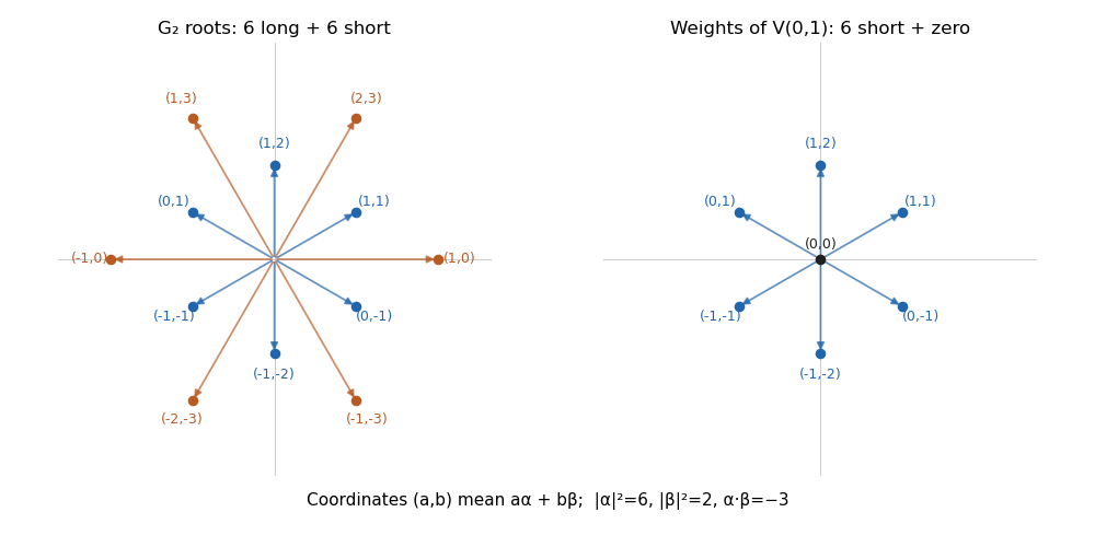
In the diagram above, a coordinate label $(a,b)$ means $a\alpha +b\beta$. The left panel contains all twelve roots of a root system; the right panel contains the six short-root weights and the zero weight. The long-root-first convention is the same as in the calculations.

Evaluate the metric inner products of the proposed orthonormal tetrad to first order in the vector cosmological perturbation:The orthonormal tetrad therefore has metric signature $(-,+,+,+)$ to the required order. Put $q=ϵ/a^2$ and $b=\mathbf{e}\cdot \mathbf{B}$. The photon momentum components areThey satisfy the null vector condition to first order, with $|\mathbf{e}|=1$.

Use $\eta$ as parameter in the time component of the geodesic equation:The derivative of the direction is first order, since the background photon moves on a straight comoving line; $B_{i}d{e}^i/d\eta$ is consequently second order. With $d\mathbf{x}/d\eta =\mathbf{e}+O(B)$,The supplied Levi-Civita connection coefficients giveThe spatial gradients and all background expansion terms cancel. Since ${ϵ}^{\prime }/ϵ$ vanishes in the background, its product with $b$ is also second order. The photon energy redshift from a vector metric perturbation is thereforeAn independent check uses the covariant component $p_0=g_{0\mu }{p}^{\mu }=-ϵ+O(B^2)$. The covariant geodesic equation gives $d{p}_0/d\eta =(2p^0{)}^{-1}{\partial }_{\eta }{g}_{\alpha \beta }{p}^{\alpha }{p}^{\beta }=ϵe^i{\dot{B}}_i$; the conformal expansion term vanishes by the null vector condition and reproduces the same result.

Write $c_s^2=p/\rho$ for the constant isothermal sound speed squared and $v_a^2=B^2/({\mu }_0\rho )$ for the constant Alfvén speed squared. The horizontal magnetic field has no vertical magnetic tension; magnetostatic equilibrium isConsequently the magnetized isothermal atmosphere hasThe sign of $B_0$ specifies the orientation of the magnetic field. The adiabatic sound speed is $v_s^2=\gamma p/\rho =\gamma c_s^2$, also constant.

For the proposed normal mode, let $A=\exp (i\mathbf{k}\cdot \mathbf{x}+z/(2H)-i\omega t)$, $a=1/(2H)$, and temporarily write $\mathbf{\xi }$ for its constant complex amplitude. The divergence amplitude is $\Delta =i{k}_x{\xi }_x+i{k}_y{\xi }_y+(i{k}_z+a){\xi }_z$. Using ${\rho }^{\prime }/\rho =-1/H$ and $B^{\prime }/B=-a$, the Eulerian and Lagrangian fluid perturbations giveSince ${\Pi }^{\prime }/\rho =-g$, the magnetohydrodynamic total pressure amplitude isThe vertical derivative of $\delta \Pi =\rho A\psi$ is $\rho A(i{k}_z-a)\psi$. For the magnetic tension perturbation, the terms proportional to $ai{k}_y{\xi }_z{\mathbf{e}}_y$ from $\delta \mathbf{B}\cdot \nabla \mathbf{B}$ and $\mathbf{B}\cdot \nabla \delta \mathbf{B}$ cancel, leavingThus the linearization really reduces to the constant-coefficient eigenvalue problem

For a static ideal magnetohydrodynamics equilibrium with conservative gravitational acceleration, the magnetohydrodynamic energy principle gives a Hermitian operator for the restoring force in the mass density weighted inner product, provided the surface terms vanish. The factor $e^{z/(2H)}$ removes the exponential mass density weight. This can be checked directly, without assuming stability: set $s=v_s^2$, $b=v_a^2$, and $q=s+b$. Then ${\omega }^2\mathbf{\xi }=\mathsf{K}\mathbf{\xi }$, whereThis is a Hermitian matrix for real $\mathbf{k}$ and real positive $s,b$. Therefore every squared frequency ${\omega }^2$ is real; negative values give exponential growth, rather than an oscillation with a complex squared frequency. In an infinite atmosphere these are generalized plane waves, not finite-total-energy global modes.