Short options paper shared by Parts A and B of the physics course of the University of Oxford

A single booklet shared by Parts A and B. The 2019 cover explicitly lists both parts; candidates answer questions from the short options for which they have entered.

Source paper: www.whatdotheyknow.com/request/oxford_physics_past_papers_2/response/2340696/attach/7/Physics%20Papers%202018.pdf?cookie_passthrough=1#page=114

The dated cover identifies this as the 2019 shared Parts A/B booklet; the public bundle filename says 2018. Solutions cover every option. Numerical estimates use stated modelling assumptions.

A complex derivative computed along the real and imaginary directions gives $f^{\prime }=u_x+i{v}_x=v_y-i{u}_y$. Equality yields the Cauchy-Riemann equationsThe gradients satisfy $\nabla u\cdot \nabla v=u_x{v}_x+u_y{v}_y=0$. Since a gradient is normal to a regular level set, the two families meet at right angles by orthogonality wherever $f^{\prime }\ne 0$. At a critical point the regular-curve argument fails: for $f=z^2$ both gradients vanish at zero, so the assertion requires this qualification.

Set $A=x^2-y^2$ and $B=2xy$. Direct differentiation givesTheir sum vanishes, proving that $u$ is a harmonic function. More generally the Cauchy-Riemann equations give $u_{xx}+u_{yy}=v_{yx}-v_{xy}=0$ and $v_{xx}+v_{yy}=-u_{yx}+u_{xy}=0$; the mixed partial derivatives commute because a holomorphic function is smooth. Since $e^{i{z}^2}=e^{-B}(\cos A+i\sin A)$, a harmonic conjugate and the resulting holomorphic function areThese expressions also verify the Cauchy-Riemann equations directly.

The chain rule in polar coordinates gives $u_r=u_x\cos \theta +u_y\sin \theta$ and $u_{\theta }=r(-u_x\sin \theta +u_y\cos \theta )$, with analogous expressions for $v$. Substituting the Cauchy-Riemann equations givesThe restriction excludes the coordinate singularity at the origin.

Choose a continuous branch of a multivalued function of the complex logarithm on a simply connected region avoiding zero. ThenAlternatively $u_r=-e^{-\theta }\sin (\ln r)/r=v_{\theta }/r$ and $v_r=e^{-\theta }\cos (\ln r)/r=-u_{\theta }/r$, verifying the Cauchy-Riemann equations. The holomorphy is local to a chosen branch of a multivalued function: increasing $\theta$ by $2\pi$ multiplies $g$ by $e^{-2\pi }$, so this is not a single-valued holomorphic function on the whole punctured plane.

For $n\ge 1$, $f=z^n{e}^{n/z}$ is holomorphic at every finite nonzero point. At zero its Laurent series has infinitely many negative powers, so zero is an essential singularity. If the Riemann sphere is included, $f(1/w)=w^{-n}{e}^{nw}$ has a pole of order $n$ at $w=0$, so infinity is a pole of order $n$.

Expanding the exponential function produces the Laurent seriesIn particular its residue is $a_{-1}=n^{n+1}/(n+1)!$.

For a positively oriented circle of any radius $R>0$, the residue theorem givesOnly the $z^{-1}$ coefficient in the Laurent series contributes. Reversing the orientation changes the sign.

If $f(z)=\sum a_j{z}^j$, then $f(-z)=\sum (-1{)}^j{a}_j{z}^j$ and its residue at zero is $-a_{-1}$. The circle $|z-1|=2$ encloses zero and no other finite singularity. Thus the residue theorem givesfor positive orientation.

Cauchy's integral theorem states that a holomorphic function on a simply connected open region has zero contour integral around every closed piecewise smooth contour in that region. More generally the same holds for a contour homologous to zero in its domain of holomorphy. Having no singularity on the curve alone is insufficient: $1/z$ has a nonzero contour integral around the unit circle.

Put $z=e^{i\theta }$, so $d\theta =dz/(iz)$, $\cos 2\theta =(z^2+z^{-2})/2$ and ${\cos }^{2}3\theta =(z^6+2+z^{-6})/4$. The contour integral isThe enclosed poles are $0$ and $\pm 1/\sqrt{2}$. For the rational function displayed without the prefactor $1/(4i)$, the residue at zero is $-21/8$ and the two other residues sum to $27/8$. Therefore the residue theorem givesA useful independent check is the Fourier series $(5-4\cos \varphi {)}^{-1}=\frac{1}{3}[1+2{\sum }_{k\ge 1}{2}^{-k}\cos k\varphi ]$; only its constant and third Fourier coefficients survive.

The square root produces branch points at $z=\pm 1$, with local behaviour proportional to $(z\mp 1{)}^{-1/2}$. One branch cut can join them along $[-1,1]$. Another choice uses the two rays $(-\infty ,-1]\cup [1,\infty )$. Each choice prevents a loop from enclosing just one branch point within a single-valued domain. For the finite-segment choice fix $\sqrt{z^2-1}\sim z$ at infinity. Infinity is then a pole of order three, not a branch point, since

Use the branch cut $[-1,1]$ and the branch of a multivalued function normalized by $\sqrt{z^2-1}\sim z$. The Laurent series from the preceding solution has $z^{-1}$ coefficient $3/8$. Consequently every sufficiently large positively oriented circle givesAlthough $f$ grows cubically, its other Laurent series terms have zero contour integral. Choosing the opposite branch of a multivalued function reverses the sign; neither the branch of a multivalued function nor the orientation can be omitted from the answer.

Shrink the positive outer contour to the branch cut $[-1,1]$. On its upper bank the chosen branch of a multivalued function has $\sqrt{x^2-1}=i\sqrt{1-x^2}$ and on the lower bank it has the negative of this value. The upper bank runs from $1$ to $-1$, and the lower bank runs from $-1$ to $1$. The endpoint circles contribute $O(\sqrt{ϵ})$ and vanish. HenceThe change of variables $x=\sin t$ independently reduces the result to the integral of ${\sin }^{4}t$ over $[-\pi /2,\pi /2]$.

Kepler's third law for two point masses in a Newtonian gravitational field isHere $a$ is the semimajor axis of their relative orbit, $P$ the orbital period and $G$ the gravitational constant. Equivalently $(P/\mathrm{yr}{)}^2=(a/\mathrm{AU}{)}^3/[(M_1+M_2)/M_{\odot }]$, to the accuracy with which these astronomical units normalize the solar mass.

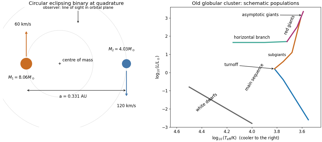
Assume a circular orbit and an orbital inclination $i\simeq 90^{\circ }$, as appropriate for a simple eclipsing binary estimate. At quadrature the two radial velocities are opposite and equal to the orbital speeds. The more massive component has the smaller amplitude. With the centre of mass as origin,Thus $a_1=0.1103\mathrm{AU}$, $a_2=0.2206\mathrm{AU}$ and Kepler's third law givesThe orbital plane contains the observer's line of sight; at quadrature the two velocities point towards and away from that observer, as labelled in the original schematic below. For an elliptic orbit, the measured amplitudes instead give $a\sin i=P(K_1+K_2)\sqrt{1-e^2}/(2\pi )$; the numerical answer requires the circular assumption.

Adopt the approximate mass-luminosity relation $L/L_{\odot }\simeq (M/M_{\odot }{)}^3$ and equal available fuel fractions. The main-sequence lifetime then scales as $M/L$, givingUsing an exponent $3.5$ instead gives about $5.4\times 10^7$ and $3.1\times 10^8$ years; these are model-dependent estimates. At $r=3r_s=6GM/c^2$ the Newtonian gravitational potential energy released from infinity is $GMm/r=m{c}^2/6$. Half remains as kinetic energy in a circular orbit, so the radiatable binding energy is $GMm/(2r)$:Using the whole potential energy loss would give $1/6$, which does not subtract the final kinetic energy. A fully relativistic calculation for a nonrotating black hole gives $1-\sqrt{8/9}\simeq 5.7\%$. When the surviving star exhausts hydrogen burning, it expands off the main sequence and can fill its Roche lobe. Binary mass transfer to the black hole can form an accretion disk and an X-ray binary; unstable binary mass transfer may instead produce a common envelope. This is conditional on the binary star remaining bound after the first remnant forms. The supplied black hole endpoint is an assumption, not a universal outcome for an isolated $8M_{\odot }$ star.

A thin spherical shell has outward pressure force $-4\pi r^2(dP/dr)dr$ and inward gravitational force $GM(r)4\pi r^2\rho (r)dr/r^2$. Hydrostatic equilibrium requiresA uniform-density solar model gives $M(r)=M_{\odot }(r/R_{\odot }{)}^3$, $\bar{\rho }=3M_{\odot }/(4\pi R_{\odot }^3)$, and after integration from $R_{\odot }$ to zero,Thus the appropriate orders of magnitude are $10^{14}$–$10^{16}\mathrm{Pa}$ and $10^7\mathrm{K}$. The uniform-density approximation underestimates the actual central pressure because the Sun is centrally concentrated. Radiation pressure is neglected in applying the ideal gas law.

A free-fall timescale estimate follows from $R/t^2\sim GM/R^2$:Falling to a central point mass gives the more precise factor $\pi /(2\sqrt{2})$, or $1.77\times 10^3\mathrm{s}$; a distributed star changes an order-one coefficient. For any spherical mass distribution with radius $R$,The inequality is strict for an extended star; equality is approached by a thin shell at $R$. For an monatomic gas the virial theorem is $2U+\Omega =0$, so half the gravitational potential energy released by contraction heats the star and half can be radiated. The Kelvin-Helmholtz cooling time is therefore of orderA uniform-density model gives $3G{M}^2/(10RL)\simeq 9.4\times 10^6\mathrm{yr}$. The given bound fixes a scale, rather than an exact contraction history; both estimates are far shorter than the Sun's main-sequence lifetime.

The right panel of the figure in solution has luminosity increasing upwards and effective temperature decreasing to the right. An old globular cluster contains a low-mass main sequence, a main-sequence turnoff, subgiants, a red giant branch, a horizontal branch, an Asymptotic giant branch and a faint hot white dwarf sequence. Its high-mass main sequence is absent because those stars have evolved.

If a fraction $f_c=0.1$ of the star participates in hydrogen burning, with initial hydrogen mass fraction $X=0.7$, the available nuclear binding energy is $0.007f_{c}XM{c}^2$. Assuming a roughly constant luminosity and coeval stars,Taking the quoted core fraction as hydrogen fuel itself, $f_{c}X=0.1$, gives $1.98\times 10^{10}\mathrm{yr}$. Stating the fuel convention matters: burning the whole stellar mass overestimates the age by about an order of magnitude. Evolving luminosity and detailed stellar structure are needed for an accurate age.

The Milky Way has a thin stellar galactic disk, radius roughly $15$–$20\mathrm{kpc}$ and scale height about $0.3\mathrm{kpc}$, containing gas, dust, young and old stars, spiral arms and most current star formation. Its stellar mass is a few $10^{10}{M}_{\odot }$. A thicker, older galactic disk has scale height around $1\mathrm{kpc}$ and stellar mass of order $10^{10}{M}_{\odot }$, with little cold gas.

The central galactic bulge and bar extend a few thousand parsecs and contain about $10^{10}{M}_{\odot }$, largely older stars. The central supermassive black hole has mass about $4\times 10^6{M}_{\odot }$ and is negligible in the total galactic budget. A diffuse old metal-poor stellar halo, extending tens to over $100\mathrm{kpc}$, contains globular clusters and roughly $10^9{M}_{\odot }$ in stars. An extended dark matter halo reaches roughly $200\mathrm{kpc}$ and dominates the total mass, of order $10^{12}{M}_{\odot }$. These are approximate component scales; the gaseous galactic halo also extends beyond the stellar galactic disk.

Treat the gravitational field as approximately spherical. The circular orbit condition givesIf every star had a representative mass $m$ and obeyed $L/L_{\odot }=(m/M_{\odot }{)}^3$, its mass-to-light ratio would be $(m/M_{\odot }{)}^{-2}$, giving $\boxed{m\simeq 0.47M_{\odot }}$. This is a one-mass estimate, not an actual average inferred uniquely from the data: a galactic stellar mass function, stellar remnants, dust and nonstellar mass alter the relation. The flattening of the galactic disk also changes the spherical conversion by an order-one factor.

Assume an isotropic, stationary spherical galaxy cluster. Its three-dimensional velocity dispersion obeys $⟨v^2⟩=3{\sigma }_{\mathrm{los}}^2$. For a uniform sphere, the virial theorem gives $3M{\sigma }_{\mathrm{los}}^2=3G{M}^2/(5R)$, henceA different density profile changes the coefficient, so $10^{15}{M}_{\odot }$ is the meaningful scale. For isothermal X-ray gas in hydrostatic equilibrium,Using $\mu =0.6$ and a representative slope $-d\ln {\rho }_g/d\ln r=2$–$3$ at $1\mathrm{Mpc}$ gives $M_X\simeq (1.3$–$1.9)\times 10^{15}{M}_{\odot }$. The temperature and extent alone cannot fix this coefficient without a density profile. The total luminosity is $5\times 10^{12}{L}_{\odot }$, so the previously inferred mass-to-light ratio gives

Three physically distinct contributions are unseen dark matter, hot diffuse intracluster gas omitted from the summed stellar mass, and faint stars or stellar remnants missed by transferring the Milky Way mass-to-light ratio to the cluster. The first two are actual additional components; the third changes the inferred stellar budget. Departures from virial equilibrium, velocity anisotropy or extra nonthermal pressure can also bias the dynamical or X-ray estimates, although they need not remove the discrepancy.

Define the canonical momentum $p_i=\partial L/\partial {\dot{q}}_i$ and the energy function $E={\sum }_i{p}_i{\dot{q}}_i-L$. Along an Euler-Lagrange equation solution,Thus an autonomous Lagrangian has conserved $E$. For a simple harmonic oscillator, $L=m{\dot{x}}^2/2-k{x}^2/2$ and $\boxed{E=m{\dot{x}}^2/2+k{x}^2/2}$ is constant. For ordinary time-independent mechanical coordinates this is the total mechanical energy.

The appropriate invariance is invariance of the action element $Ldt$, including the change of the time measure. Under $\delta t=\lambda \varphi$ and $\delta q_i=\lambda {\psi }_i$, differentiation of $q_i^{\prime }(t^{\prime })$ gives $\delta {\dot{q}}_i=\lambda (D_t{\psi }_i-{\dot{q}}_i{D}_t\varphi )$. ThereforeUsing the Euler-Lagrange equations and $D_{t}E=-L_t$, this becomesAn action symmetry therefore yields the Noether chargeFor $\varphi =0$ this reduces to the usual spatial form of Noether's theorem. The same on-shell calculation permits velocity-dependent generators when they define a legitimate variational symmetry. Merely preserving the numerical value of $L$ is insufficient for transformations of time: the Jacobian matrix and determinant $d{t}^{\prime }/dt$ matters. If the action changes by a boundary term $\lambda D_{t}B$, the conserved quantity is $Q-B$.

For a central potential use $L=m|\dot{\mathbf{r}}{|}^2/2-V(|\mathbf{r}|)$. An infinitesimal rotation about any constant unit vector $\mathbf{n}$ has $\varphi =0$ and $\mathbf{\psi }=\mathbf{n}\times \mathbf{r}$. Noether's theorem gives $Q=m\dot{\mathbf{r}}\cdot (\mathbf{n}\times \mathbf{r})=\mathbf{n}\cdot \mathbf{L}$, where $\mathbf{L}=\mathbf{r}\times m\dot{\mathbf{r}}$. Since $\mathbf{n}$ is arbitrary, every component of angular momentum is conserved. A time-translation symmetry has $\varphi =1$, $\mathbf{\psi }=0$, giving $Q=-E$ andas conserved quantities.

The orbiting planet produces a potential $V(r,\vartheta ,\phi -\Omega t)$. It has explicit time dependence and exerts an azimuthal torque, so generally $\dot{E}=V_t$ and ${\dot{L}}_z=-V_{\phi }$ are nonzero. Nevertheless a simultaneous time-translation symmetry $\delta t=\lambda$ and rotation $\delta \phi =\Omega \lambda$ leaves the Lagrangian and $dt$ unchanged. Noether's theorem gives $Q=\Omega p_{\phi }-E$ and henceEquivalently $V_t=-\Omega V_{\phi }$ implies $d(E-\Omega L_z)/dt=0$. This Jacobi integral assumes a rigidly rotating potential with constant $\Omega$ and negligible back-reaction from the test particle.

Write the geometric vector as $\mathbf{V}={\sum }_i{V}_i^{\prime }{\mathbf{e}}_i^{\prime }(t)$. A rotating orthonormal basis obeys ${\dot{\mathbf{e}}}_i^{\prime }=\mathbf{\Omega }\times {\mathbf{e}}_i^{\prime }$. The product rule gives the transport identityBoth terms must be expressed in the same basis before adding them. If $R(t)$ maps rotating components into inertial components, the precise component equation is $d(R{\mathbf{V}}^{\prime })/dt=R({\dot{\mathbf{V}}}^{\prime }+{\mathbf{\Omega }}^{\prime }\times {\mathbf{V}}^{\prime })$. The printed expression suppresses this basis conversion.

The inertial Lagrangian is $L=m|\dot{\mathbf{r}}{|}^2/2-U(\mathbf{r},t)$. Put $\mathbf{r}=R(t){\mathbf{r}}^{\prime }$ and define $U^{\prime }({\mathbf{r}}^{\prime },t)=U(R(t){\mathbf{r}}^{\prime },t)$. The transport identity and invariance of the Euclidean norm under a rotation giveIts expansion contains the ordinary kinetic energy, $m{\dot{\mathbf{r}}}^{\prime }\cdot ({\mathbf{\Omega }}^{\prime }\times {\mathbf{r}}^{\prime })$, and $m|{\mathbf{\Omega }}^{\prime }\times {\mathbf{r}}^{\prime }{|}^2/2$. These velocity and position terms generate the apparent forces in the rotating frame.

Suppress primes on the angular velocity while retaining rotating components. The canonical momentum is $\partial L^{\prime }/\partial {\dot{\mathbf{r}}}^{\prime }=m({\dot{\mathbf{r}}}^{\prime }+\mathbf{\Omega }\times {\mathbf{r}}^{\prime })$. Varying $L^{\prime }$ with respect to position and applying the Euler-Lagrange equations givesThe terms are the physical force, the velocity-dependent Coriolis force, the outward centrifugal force, and the Euler force caused by changing angular velocity. The common origin is inertial; an accelerating origin would introduce another translational apparent force.

At latitude $\ell$, the Earth's angular velocity in east–north–up coordinates is $\mathbf{\Omega }=(0,\Omega \cos \ell ,\Omega \sin \ell )$. Assume a small horizontal patch, constant $\Omega$, negligible vertical velocity, and a vertical constraint balancing effective gravity. Absorb the steady centrifugal force into that effective gravity. With $f=2\Omega \sin \ell$ and physical horizontal force per unit mass $F_x^{\prime },F_y^{\prime }$, the Coriolis force givesLarge-scale atmospheric and oceanic flows deflect to their right in the northern hemisphere and left in the southern hemisphere; their balance with a horizontal pressure gradient produces geostrophic flow. A Foucault pendulum has an oscillation plane that precesses relative to the ground at angular rate $-\Omega \sin \ell$. Both effects vanish at the equator within this horizontal approximation.

Let $m$ be the ice mass for which the stated drag coefficients are defined, $K=k_1+k_2$ and $f=2\Omega \sin \ell$. With stationary water, the steady horizontal ice equations areThe linear system givesFor fixed wind speed $V=10\mathrm{m}{\mathrm{s}}^{-1}$, the Cauchy-Schwarz inequality minimizes this component whenThus the wind must blow towards a direction east of south by ${\tan }^{-1}(mf/K)$ in the northern hemisphere, west of south in the southern hemisphere, and due south at the equator. This compensates the Coriolis force; at the optimum $v_x=0$ and the ice moves due south. If the drag coefficients are per unit mass, replace $K/m$ by the corresponding total drag rate. “Blows towards” avoids the opposite convention used when naming winds by their origin.