Fluid dynamics studies the motion of liquids and gases, including the forces and transport processes that determine their evolution. Its central variables include velocity, pressure, mass density and temperature, all varying with position and time.
Conservation of mass gives the continuity equation. Combining Newton's second law with a constitutive model for viscous stress gives the Navier-Stokes equations. The relative importance of inertia and viscosity, measured by the Reynolds number, explains why slow flow around a microscopic particle differs so sharply from a turbulent river. Boundary conditions and material properties are essential parts of a fluid model.
A flow containing two or more distinguishable material phases, such as two immiscible liquids or a gas-liquid mixture. Each phase can have its own volume fraction, density and velocity. Cross-sectional or ensemble averaging produces coupled phase balance equations whose mass, momentum and energy exchange terms must be specified consistently. A common pressure alone does not automatically make an averaged model well posed.
Take incompressible phase mass equations for fractions and momentum equations with a common pressure. At a uniform state with , elimination of the mass and momentum perturbation amplitudes givesIts roots are the displayed speeds, whose imaginary parts are . A nonzero slip velocity therefore gives a Fourier branch growing as . No finite-order Sobolev estimate can control all high wavenumbers, showing ill-posedness of this unregularized closure. At zero slip the roots coincide and this nonreal-root argument no longer settles the degenerate case. Phase-fraction endpoints also lie outside the root formula's derivation.
Here means integration over a fixed pipe cross-section divided by its area, and is the indicator of one immiscible fluid. The volume fraction is ; intrinsic density averages over the phase-occupied area rather than over the whole section. The velocity must be density-weighted for its product with mean phase density to represent mass flux exactly.
If there is no interphase mass transfer, integrating over a section with impermeable outer wall gives . The second phase uses and its own intrinsic averages. For constant phase density the velocity reduces to the ordinary phase-area average. These definitions apply where the corresponding phase fraction is positive; zero-fraction intrinsic quantities need a separate convention.
For an incompressible phase, this coefficient compares its actual axial momentum flux with the uniform-profile flux at the same intrinsic mean velocity. Cauchy-Schwarz gives where the mean is nonzero. A spatially varying profile can have a larger second moment even when its mean speed is unchanged.
With constant , expansion of and use of gives . Thus a profile correction changes both convection and phase-fraction-gradient coupling in the averaged momentum equation. If varies, an extra remains; a zero mean should be treated through the undivided second moment rather than an undefined coefficient.
The source is the mass gained by phase per mixture volume and time, through processes such as evaporation or condensation. Internal exchange conserves total mass, so its phase sources sum to zero. In an immiscible material-interface model without phase change, every is zero. The interface may still move: absence of transfer means that mass does not cross it relative to its own motion.
Laminar flow is a regime of fluid flow in which the motion remains organized, with neighboring fluid parcels following smooth, coherent paths rather than the irregular interacting fluctuations characteristic of turbulence. In a straight pipe, the simplest example consists of coaxial layers sliding past one another. This describes the character of the motion, not a requirement that every parcel have the same velocity. Nor does it require steady flow: a smooth profile can evolve in time as viscosity transmits motion from a newly moving wall into a resting fluid. The unsteady wall-driven solution provides an explicit example. [ref]
https://notes.shreyasmandre.com/fluid-dynamics-notes/Ch3.html. Shreyas Mandre, Fluid Dynamics Lecture Notes, section 3.3
The Reynolds pipe-and-dye experiment makes this distinction visible. A thin injected dye band can remain coherent in laminar flow, whereas irregular motion can fold it and carry dye across the pipe. However, molecular diffusion can spread dye even in laminar flow, and an inlet disturbance can move a coherent band without producing turbulence. A dye band is a streakline, not a measurement of the entire velocity field; in steady flow an ideal passive tracer's streakline coincides with a streamline. Reynolds explicitly distinguished a wandering band from one broken into eddies. [ref]
https://archive.org/stream/philtrans06508925/06508925_djvu.txt. Osborne Reynolds, An Experimental Investigation (1883), section 11, pp. 941–943
For a circular pipe of internal diameter , define the mean axial velocity using the volumetric flow rate and cross-sectional area :Here is mass density, is dynamic viscosity and is kinematic viscosity. This particular Reynolds number uses the diameter and mean velocity, not the radius or centreline velocity. Small Reynolds number generally favors laminar flow, but a single universal critical Reynolds number does not distinguish it from turbulence in all geometries and experiments. Even in a given pipe, inlet conditions and the magnitude of disturbances affect the observed onset. Reynolds demonstrated this dependence by deliberately inserting a wire coil. [ref]
https://archive.org/stream/philtrans06508925/06508925_djvu.txt. Osborne Reynolds (1883), section 23, pp. 955–956
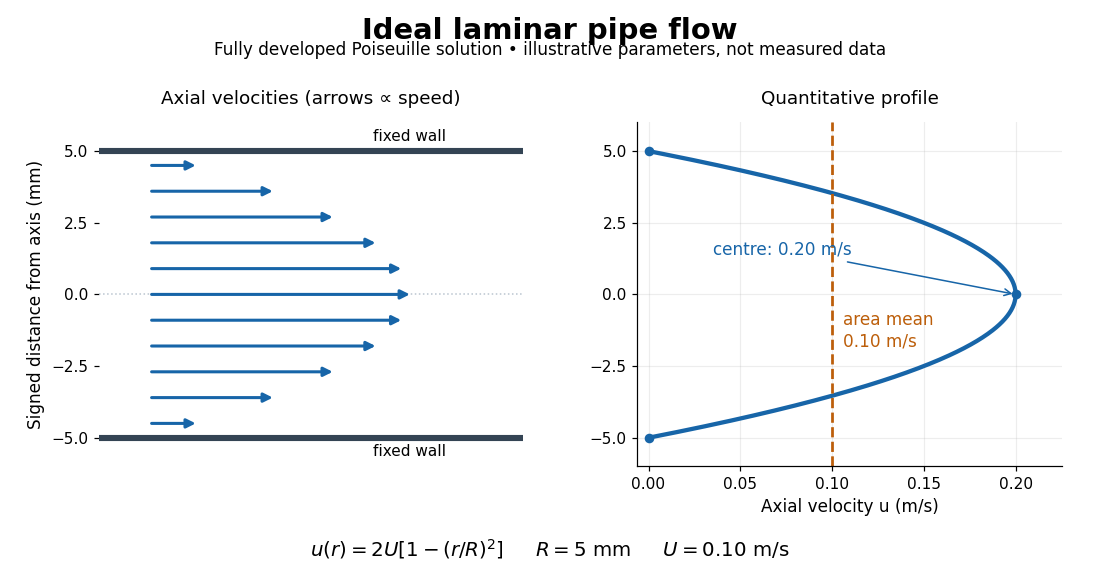
The quantitative example above assumes steady flow, incompressible flow, a Newtonian fluid with constant dynamic viscosity, a straight horizontal circular pipe of radius , stationary walls satisfying the no-slip boundary condition, and fully developed flow. The last assumption means that the axial velocity profile no longer changes downstream. A positive pressure drop over a developed length gives the Hagen-Poiseuille equation:The velocity is zero at the wall and maximal at the centre. Averaging over the circular area, whose annuli have area , gives ; averaging along one diameter would give a different answer. These assumptions produce a parabola, rather than every laminar flow having a parabolic profile. [ref]
https://notes.shreyasmandre.com/fluid-dynamics-notes/Ch3.html. Shreyas Mandre, Fluid Dynamics Lecture Notes, section 3.2.2, equations (3.9)–(3.11)
As a stipulated calculation, take , , , and , and assume the developed laminar flow above. Then , , , (about ), and . These are predictions from chosen parameters, not measurements or a claim that guarantees laminar flow in every apparatus.
The beauty of this example is that a spatially varying velocity field still gives an exact relation between two accessible measurements, pressure drop and volumetric flow rate. It predicts the hydraulic resistance . Doubling the radius therefore multiplies by sixteen at fixed pressure drop, length and dynamic viscosity, provided the model remains applicable. This makes the laminar flow model useful for sizing narrow tubes or determining dynamic viscosity. It also explains why a persistent narrow dye band can be informative without implying that the fluid is moving as a uniform plug.
In his 1883 paper, Osborne Reynolds investigated how the character of pipe flow depends jointly on velocity, pipe diameter and viscosity. His final dye apparatus drew water from a large glass tank through a horizontal glass tube with a smooth trumpet-shaped entrance. A separate reservoir supplied strongly colored water just upstream of the entrance; a valve below the tank controlled the outflow. The glass tube was immersed in the tank, so its internal dye band could be watched. Reynolds repeated the trials with different tube diameters and water temperatures. [ref]
https://archive.org/stream/philtrans06508925/06508925_djvu.txt. Osborne Reynolds (1883), sections 11 and 21–22, pp. 941–943 and 951–953
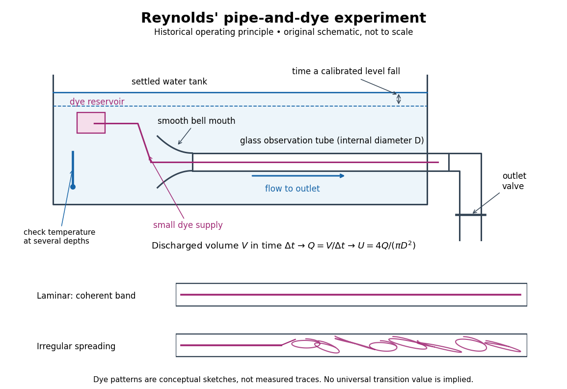
Reynolds' pipe-and-dye experiment: observe the dye while measuring discharge and temperature
. Original schematic of the historical operating principle, not a scale reconstruction. A falling tank level determines discharged volume; timing it gives flow rate. The lower dye patterns are conceptual sketches of a coherent band and irregular spreading, not measured trajectories or concentration records. Details.The volumetric flow rate was measured independently of the appearance of the dye. Reynolds timed a one-inch fall of the tank's water level, corresponding to a calibrated discharged volume. In modern notation, if this volume is and the elapsed time is , then and . He determined the glass tubes' internal diameters by filling them with water. For a uniform bore, a known filled length and measured water volume determine ; checking bore uniformity matters because the same volume would only give an average cross-section in a tapered tube. Thermometers at different tank levels checked both the temperature and its uniformity. Reynolds compared the viscosity at different temperatures using Poiseuille's results and checked his own water by separate experiments of that type. Thus the Reynolds number estimate did not come from judging the dye band or from assuming that transition occurred at a preset value. [ref]
https://archive.org/stream/philtrans06508925/06508925_djvu.txt. Osborne Reynolds (1883), sections 21–22 and the reductions following Table I, pp. 951–955
A practical repetition can instead collect a known outflow volume in a measuring vessel and time its collection, or weigh the collected water and divide its mass by mass density. Measure the internal diameter, rather than the external diameter, and obtain kinematic viscosity at the measured water temperature from independently established properties or a separate viscosity measurement. Record the dye appearance and observation position alongside , , temperature and the resulting Reynolds number. These are alternative measurement procedures following , not additional historical claims about Reynolds' dye apparatus.
Begin with settled water and a small dye supply, then open the outlet valve in small steps. Reynolds saw a thin straight band at sufficiently low speeds. With a tank that had not fully settled, the band could wander while retaining its coherence. At higher discharge it could abruptly spread into the surrounding water downstream of the entrance. Short illumination by an electric spark resolved curls within what otherwise looked like a colored cloud. This connected the visible breakup with internal irregular motion rather than merely the appearance of an opaque pipe. [ref]
https://archive.org/stream/philtrans06508925/06508925_djvu.txt. Osborne Reynolds (1883), sections 11 and 22, pp. 942 and 951–952
The controls are part of the result. Reynolds used a smooth entrance and let the tank rest to reduce inlet disturbances. He found that a heated tank could retain slow circulation as it cooled, so measuring one temperature was insufficient: thermal uniformity and residual motion also mattered. His wire-coil trial broke up the band below the previous onset speed, but he explicitly cautioned that once the dye was mixed he could not tell from that dye alone whether the motion became orderly again farther along the tube. In a repetition, keep the dye supply small enough to act approximately as a passive scalar, avoid a strong injection jet, and record the inlet condition and downstream observation distance. If also testing the Hagen-Poiseuille equation, allow the profile to develop and measure pressure drop between positions within the developed region; do not treat the entrance and outlet losses as part of its uniform pressure gradient. The dye experiment by itself does not establish fully developed flow. [ref]
https://archive.org/stream/philtrans06508925/06508925_djvu.txt. Osborne Reynolds (1883), sections 21–23 and 26, pp. 951–956 and 959
The experiment's usefulness is that it compares a visible change in the motion with independently measured scales. Repeating it with several diameters and temperatures, while controlling disturbances, tests the organizing role of the Reynolds number. Its limitations are equally instructive: dye is a tracer of transport, diffusion still acts in laminar flow, and a local dye observation cannot by itself prove that turbulence persists throughout an arbitrarily long pipe.
Sediment transport is movement of grains by a flowing fluid, through motion close to a bed or within a particle suspension. A flow's shear stress and fluctuating forces compete with grain weight, contacts and friction. The Shields parameter compares a bed-stress scale with the submerged grain-weight scale and helps organize the threshold for movement.
Bedload transport carries grains along or near the bed, while suspended sediment balances settling against upward mixing and entrainment. The transport budget changes the bed itself: mass conservation in the Exner equation relates downstream flux divergence to erosion or deposition. A flow entering an erodible reach can take a finite distance to establish its transported grain population, described by sediment transport saturation. These couplings make a bed an evolving part of the fluid problem rather than a fixed rough wall. Measuring both transported material and bed-height change tests whether the sediment budget closes.
In a reduced sediment-bed model with normalized discharge one, water momentum gives , while concentration adaptation and bed exchange give . Linearizing about yields and . Elimination proves the displayed dispersion relation.
For , the growth rate is , positive exactly on the supercritical side for nonzero . The phase speed is , so unstable bedforms migrate upstream and are antidunes. At high wavenumber growth approaches a finite plateau rather than becoming unbounded. This closure selects no finite fastest wavelength; short-scale selection needs additional physics. The critical limit and a vanishing entrainment derivative are degenerate cases outside the displayed conclusion.
Bedload transport is motion of sediment grains along or close to the bed, represented in a depth-averaged model by a solid-volume flux per unit width. The Exner equation balances this flux divergence and changes in porous-bed solid storage against exchange with suspended sediment. Consistent mass units are necessary when adding this equation to a suspended mass-concentration balance.
Keeping sediment acceleration while neglecting water storage and a small gravity-friction residual gives a reduced model for the bed elevation , water speed and sediment speed . A prescribed water flux gives ; integrated water momentum gives . Around the normalized uniform state , let , . A Fourier mode of wavenumber has growth-rate real partThus nonuniform modes decay for subcritical Froude number and grow for supercritical Froude number. The spatially constant mode is neutral, and the critical value needs terms neglected in this reduction. In a general uniform state the sign change is at the actual mean-flow Froude number equal to one, rather than at a velocity-scale parameter unrelated to that state.
Suspended sediment is particulate material carried within a fluid rather than solely along the bed. Its concentration balance includes advection, erosion into suspension and deposition from suspension. For water depth and suspended mass concentration , the conservative balance reduces using water continuity to .
A dune is a sediment bedform. In the elementary subcritical flow description of river dunes, bed undulations and free-surface undulations are out of phase. This phase relation identifies a hydraulic response; instability additionally requires a positive real part of the relevant dispersion relation. Contrast the in-phase surface of an antidune.
An antidune is a bedform associated with supercritical free-surface flow, in which bed and surface undulations are approximately in phase. In the elementary erodible-bed model with suspended sediment, an unstable branch can migrate upstream. Its growth and migration depend on the hydraulic and sediment-response parameters; the high-wavenumber antidune dispersion calculation makes the required supercritical regime explicit.
In the fast-water limit of an erodible-bed shallow water equations model, let , and be the suspended-load relaxation coefficient. Linearization and elimination give the dispersion relation . Its real part tends to the finite constant in the title, and phase velocity tends to . Thus the unstable upstream branch requires supercritical flow and enough sediment feedback to overcome friction; subcritical flow has the opposite propagation sign and decay at leading order. The near-critical limit needs a separate balance.
Sediment resuspension transfers deposited bed particles into a particle suspension. It can supply particle buoyancy flux to a particle-laden gravity current if erosion or upward mixing exceeds settling losses. Ambient fluid without particles dilutes concentration without supplying particle mass.
For downward settling velocity magnitude and eddy diffusivity , the total upward particle flux is . A stationary profile tending to zero at infinity has , giving the displayed power law. The exponent compares settling with turbulent mixing. It describes a region above the bed; entrainment from the bed and viscous near-wall effects determine the reference concentration separately.
Sediment transport saturation is relaxation of a transported grain population toward the equilibrium sediment flux supported by local flow conditions. A change in bed shear stress does not immediately give a fully adjusted grain speed and population. Close to equilibrium, a steady model isFor constant and saturation length , this gives . The spatial lag matters for bedform growth.[ref]
Measurements of the aeolian sand transport saturation length by Bruno Andreotti and others. §1, equation (1): near-saturation relaxation and possible limiting mechanisms
A published wind tunnel test used a wide, high and long tunnel. Repeated measurements of bed elevation after stopping the flow supplied an erosion rate; integrating that rate inferred downstream flux by mass conservation. The fitted near-equilibrium relaxation length was distinguished from the earlier grain-ejection stage, so the total development distance was not treated as the same parameter.[ref]
Measurements of the aeolian sand transport saturation length by Bruno Andreotti and others. §2, Wind tunnel measurements: geometry, elevation-based flux inference and separate ejection/relaxation stages
The equilibrium sediment flux is the transport supported locally by a prescribed bed shear stress. A common idealization is . Linearization above the sediment entrainment threshold requires perturbations small compared with the positive excess stress.
The saturation length measures downstream relaxation of a transported grain population toward its equilibrium sediment transport flux. The elementary steady relaxation law is ; it introduces a phase lag between forcing and actual transport.
The Exner equation is local sediment mass conservation expressed in terms of solid volume: accumulation raises the bed and flux divergence lowers it. Here is the solid volume fraction of the packed bed and is solid volume flux per unit width.
A leading fixed-discharge, level-surface approximation to a shallow erodible-bed flow gives perturbation equations and . The displayed Fourier growth rate has negative real part for every nonzero wave number, independently of bedload parameter . Bedload changes the propagation speed but not this damping. The zero-wave-number mode is neutral, so absence of growing modes should not be confused with strict asymptotic decay of every spatially uniform perturbation.
The Shields parameter is , comparing bed shear stress with a grain-scale submerged weight per area. Its critical value depends on the assumed drag coefficient, static friction, lift, and contact geometry.
The sediment entrainment threshold is the bed shear stress at which resting grains begin moving. An elementary force balance using spherical grains, tangential quadratic drag, and static friction gives when the drag coefficient is defined relative to the bed shear velocity.
For locally bed-tangent drag force and an upslope angle , a spherical-grain force balance gives . The small-slope term is . A horizontal drag force instead changes the normal contact force and gives a different slope correction.
A bedform is organized relief on a mobile sediment bed, such as a dune or an antidune. Its shape changes the overlying flow, which changes the shear stress and the sediment transport; erosion and deposition then feed back on the shape. The pattern is therefore a coupled fluid-and-grain response rather than simply a frozen pile of material.
For a small sinusoidal bed disturbance, an upstream lead of the forcing relative to bed height can favor growth, while sediment transport saturation introduces a downstream lag. The Exner equation converts the resulting flux divergence into bed-height change. Their combination determines both growth and migration; the direction of migration cannot be inferred from a bed's appearance alone. Recording a bed profile at successive times separates changing amplitude from movement of a crest, while flow measurements test the assumed bed shear response.
Combining the Exner equation, sediment transport saturation, bed shear response, and inclined-bed sediment threshold gives a competition between upstream forcing and downstream relaxation. With , , , and positive wavenumber , the growth rate is . Thus permits long-wave growth when , while a finite saturation length stabilizes shorter waves.
For a small sinusoidal bedform, a fluid-dynamical closure can be written for . The real coefficient is in phase with the bed height and describes an upstream phase lead. Neither coefficient follows from the Exner equation or sediment relaxation alone; they require a flow calculation or measurement.
An acoustic wave is a propagating disturbance in a material's pressure, mass density and particle motion. Compressing a small fluid region raises its pressure; the resulting pressure gradient accelerates adjacent material, while inertia carries the motion onward. This restoring mechanism permits longitudinal waves in an ordinary fluid.
For small perturbations about a uniform resting state, the linear continuity equation and momentum conservation combine into a wave equation. The squared speed of sound is the relevant derivative of pressure with respect to mass density; rapid locally reversible compression usually uses the isentropic derivative. A microphone records the pressure variation, while a travel-time measurement probes propagation speed. The particle velocity can remain much smaller than the speed of sound: local material oscillation and movement of the wave pattern are different quantities. Acoustic energy flux relates the pressure and particle-velocity fields to transported power.
For a rigid cylinder of radius and height , the velocity potential obeys the wave equation with Neumann boundary conditions. Separation in cylindrical coordinates gives radial factors , angular sine and cosine factors of integer order , and axial factors . The nonzero radial numbers satisfy , yielding the displayed frequencies.
There is also a constant radial mode, with and radial number zero. A formal zero of at the origin for higher must not be counted by substituting into , which would give the zero function. Solving the zero-radial-eigenvalue equation directly leaves only the constant mode under the side-wall condition. The fully constant potential has zero velocity and is a gauge mode; constant radial modes with nonzero axial index are physical longitudinal oscillations.
Nonlinear acoustics retains finite-amplitude effects in sound waves, including amplitude-dependent propagation speed, distortion and possible shock waves. For a one-dimensional polytropic flow with , a rightgoing simple wave has characteristic speed relative to a quiescent reference. Thus small-amplitude linear acoustics need not be uniform when a background velocity nearly cancels the speed of sound.
Ultrasound is sound above the conventional upper limit of human hearing, approximately . In a crystal, ultrasonic travel-time measurements determine long-wavelength elastic wave speeds, which are the small-wavevector slopes of the corresponding acoustic phonon branches.
Acoustic measurement of a moving-scatterer velocity projection using frequency or phase changes. A speed estimate needs the scattering geometry; finite pulsed sampling can alias the measured shift.
An emitted acoustic pulse is followed by detection of returning echoes. Travel time estimates depth under a declared sound-speed and path model, while echo amplitudes depend on interfaces and propagation losses.
An M-mode ultrasound scan repeatedly samples one pulse-echo ultrasound beam and places successive depth profiles alongside one another in time. Depth is one display axis and acquisition time the other; echo strength controls brightness. This makes motion along the selected line visible. [ref]
A stationary interface traces a line at constant depth; an oscillating interface traces a varying depth. Converting echo delay to depth still assumes a sound speed and a return path. This display records one beam over time, whereas a B-mode ultrasound scan combines beam lines across space.
A B-mode ultrasound scan maps echo strength to displayed brightness and assembles multiple pulse-echo ultrasound lines into a spatial image. Each echo's location is inferred from beam direction and return time using an assumed sound speed. [ref]
A bright point represents a strong received echo, not a direct measurement of tissue density. Acoustic impedance contrasts, propagation losses and the instrument's display mapping all affect brightness. A moving image consists of repeated spatial frames; in an M-mode ultrasound scan, the second display axis instead tracks time along one beam.
An A-mode ultrasound scan plots the returning echo amplitude along one pulse-echo ultrasound beam. With assumed sound speed , echo delay is converted to depth by ; the factor two accounts for outward and return travel. Peaks mark reflecting interfaces along that line. [ref]
The horizontal coordinate is depth inferred from travel time, while the vertical coordinate is signal amplitude. An A-mode ultrasound scan therefore provides a one-dimensional depth profile rather than the spatial cross-section assembled by a B-mode ultrasound scan.
For a pure rightgoing acoustic wave, retarded time and slow distance separate fast oscillations from nonlinear steepening. Expanding the equation of state gives . The leading perturbations satisfy . Adding the first-order mass conservation and momentum conservation equations cancels the unknown first corrections and yields the displayed viscous Burgers equation. Inviscid characteristics satisfy , ; loss of invertibility marks shock formation and the end of the smooth inviscid approximation.
A plane-parallel atmosphere with isothermal sound speed in gravity has mass density , . Above a rigid base, vertically directed adiabatic fluid perturbations satisfy and . Set and . The substitution converts finite Gaussian-weighted kinetic energy into square integrability for . Odd extension across the base and the oscillator lowering operator force to be an odd positive integer. Thus is proportional to the Probabilists' Hermite polynomial . These are vertical acoustic waves; a general stably stratified atmosphere also admits internal gravity waves with horizontal structure.
An acoustically rigid boundary has zero perturbation normal velocity. For a reflected acoustic plane wave, pressure amplitudes add in phase and the reflection coefficient is . It is the infinite-surface acoustic impedance limit. A pressure-release boundary instead fixes the pressure perturbation to zero and reflects with coefficient .
A stratified atmosphere can reflect low-frequency acoustic waves while permitting sufficiently high-frequency waves to escape. In a plane-parallel isothermal atmosphere, the angular acoustic cutoff is approximately , where is the density scale height. Its detailed form depends on the atmospheric profile and on the wave-variable approximation.
In an isothermal atmosphere with constant density scale height , the equation loses its first spatial derivative under . Direct differentiation gives . Thus a plane wave has dispersion relation , with real acoustic cutoff frequency . The cutoff term is positive; a minus sign would instead predict growing sufficiently long spatial modes. Vertical propagation requires within this ideal constant-coefficient model.
A pressure-release boundary imposes zero acoustic pressure disturbance, . The incident and reflected pressure amplitudes therefore obey , so the pressure reflection coefficient is . It contrasts with a rigid inviscid boundary, where zero normal velocity gives . A much lower normal impedance on the far side approximates the pressure-release condition.
A sonic boom is the sound associated with shock waves from a body moving at a supersonic Mach number. The weak-wave Mach cone describes a propagation geometry rather than the finite pressure signature determining the sound strength.
A shear flow has a velocity field varying across adjacent fluid layers, giving a nonzero shear rate. A parallel example is , with vertical shear . Linear shear flow has constant shear, while a shear layer concentrates the velocity change in a narrow region.
Variation of horizontal velocity with height. In a rotating balanced stratification, thermal-wind balance relates this vertical shear to a horizontal buoyancy gradient. The sign reverses when changing from upward height to downward-increasing pressure coordinate.
A renovating shear flow holds a planar shear flow fixed for an interval , then chooses a fresh orientation independently of preceding intervals. Each interval acts on a material line by a rotated copy of the displayed deformation gradient. The orientation law must be specified: independent uniformly distributed orientations define the isotropic model, whereas a biased orientation law generally gives another Lyapunov exponent.
For independent uniform orientations in a renovating shear flow, the incident angle relative to each new shear is uniform even after earlier deformations. One interval stretches a unit material line by . Write this as , where and . The angular logarithmic integral gives . Add these independent logarithmic increments to get the displayed rate. At fixed shear rate, small gives and large gives . The unique positive maximum is at , obtained from with .
The logarithm of the stretch after independent uniform renovations is a sum of independent identically distributed bounded increments. For singular stretching , , the increment has Fourier expansion , with and . Orthogonality proves the displayed variance. The central limit theorem gives an approximate central log-normal distribution of , not an exact description of extreme tails. For , both the mean and variance of are to leading order. Direct expansion of fixed-power moments gives ; in particular mean stretch grows faster than typical stretch.
A linear shear flow has velocity that varies linearly in a transverse coordinate, such as . Its velocity gradient and shear rate are spatially constant.
Drag is the component of fluid force opposing an object's motion relative to the surrounding fluid. Surface pressure and viscous shear stress both contribute; their relative importance depends on shape and flow regime. A body can therefore experience drag even if most resistance comes from an uneven pressure field rather than direct tangential rubbing.
At low Reynolds number, the Stokes drag law gives for a sphere under its creeping-flow assumptions. In many inertial regimes, a useful representation is , with a measured or modeled drag coefficient . That coefficient can vary with Reynolds number, surface condition and geometry. Towing a body while measuring force at several speeds tests which regime applies. The supplied towing power is for steady motion along the drag direction.
Lift-induced drag is the component of aerodynamic drag associated with the three-dimensional flow that supports a finite wing’s lift. The trailing vorticity produces downwash, changing the local relative-flow direction. A force approximately perpendicular to that local flow consequently has a component opposing the freestream motion. NASA’s primary account identifies the counter-rotating wingtip vortices and the downstream force component produced by their induced flow.[ref]
Induced Drag Coefficient by NASA Glenn Research Center. Air Pressure of a Wing and Induced Drag Coefficient
For a small induced angle , a force perpendicular to the local flow has freestream components and . Hence . This elementary projection explains why changing the flow direction can change drag even without adding direct viscous rubbing to that model.
A useful finite-wing model iswhere is wingspan, the wing reference area and the span efficiency factor. Use the same reference area in and , with . NASA gives this coefficient relation and aspect-ratio definition.[ref]
Induced Drag Coefficient by NASA Glenn Research Center. Drag Coefficient, displayed Cdi and AR equations
It is a model of the induced contribution, not a statement that total drag has only this dependence in every flow regime.An original fixed-lift calculation eliminates the coefficients:Take , , , , and . Then , , , and . The corresponding induced-power contribution is . Doubling the speed while holding lift, span, density and efficiency fixed reduces this modeled drag to about .
What is held fixed matters. At fixed instead of fixed lift, induced drag grows with dynamic pressure. The familiar inverse-square-speed conclusion above therefore cannot be transferred to a test that holds angle of attack or coefficient fixed while changing speed. Changes in efficiency, separation or compressibility can also invalidate the assumed comparison.
Lifting-line theory relates spanwise loading, trailing vorticity and induced velocities. The ideal planar minimum for fixed lift and span has elliptic span loading; this is a statement about the load distribution, not merely the outline of the wing. Total drag measurements also contain profile and other contributions, so fitting a total-drag curve does not automatically isolate .
A proposed wind-tunnel study measures force components and freestream conditions for several lift settings, while separately accounting for support loads, wall effects and profile drag. A downstream velocity survey tests the predicted downwash structure. Force balance alone observes total aerodynamic loads; the split into induced and other drag requires the additional flow information or a justified model. Report those assumptions before inferring an efficiency factor from the measured drag.
Downwash is a downward component of fluid velocity, commonly the induced flow associated with a lifting wing and its trailing vortices. For positive upward lift, this flow changes the direction of the local relative wind and contributes to lift-induced drag. NASA's primary explanation connects the trailing vortex system, reduced effective incidence and rearward component of the aerodynamic force.[ref]
Choose streamwise velocity and let denote downward induced speed at a section. The induced angle and effective angle of attack areAn ideal local lifting force normal to that relative flow is tilted rearward. Its vertical and downstream projections obey ; hence for small induced angles. This projection isolates the induced contribution in the stated model; it does not include skin friction or every source of total drag.
For an original uniform-downwash example, take , and total lift . Then and in the projection model. The power required to overcome this contribution is . At geometric incidence , the effective incidence is about .
A real finite wing generally has span-dependent loading and induced speed. In small-angle lifting-line theory,Using an unweighted arithmetic mean of measured need not reproduce that integral. For elliptic span loading, the ideal lifting-line downwash is constant across the span and , consistent with . These statements concern the ideal planar model rather than arbitrary wakes or separated flow.
A proposed observation measures flow direction and speed at a specified plane around a loaded wing, using calibrated directional probes or timed tracer images. Repeat with zero and reversed lift, and compare the sign and spatial distribution of the induced flow. Record the freestream reference and wing incidence as well as the probe positions. Wake-plane dependence of a downwash measurement matters: a velocity measured well downstream cannot simply be inserted as the wing-section induced speed without a model connecting the two planes. Visible tracer deflection demonstrates flow direction only to the extent that the tracer follows the fluid; it is not by itself a quantitative lift or drag measurement.
Wake-plane dependence of a downwash measurement means that a measured downward velocity depends on where the observation plane lies relative to the lifting wing and its evolving wake. The induced velocity entering a wing-section force calculation is not generally equal to a downstream probe reading. Classical lifting-line theory explicitly adjusts local incidence using the induced flow at the lifting line, under assumptions such as steady flow, incompressible flow and a nearly planar high-aspect-ratio wing.[ref]
Prandtl's Lifting Line Introduction (16.100) by MIT OpenCourseWare. printed pp. 1–3, assumptions, induced angle and circulation equation
An original straight-filament model isolates one reason for the difference. Consider a vortex filament of circulation magnitude starting at streamwise coordinate zero and extending downstream forever. At a point with streamwise coordinate and perpendicular distance , its induced azimuthal speed isThe integral follows by differentiating . At , only one half of the corresponding infinite straight filament contributes; far downstream, the local filament extends far in both axial directions relative to .
For two straight trailing filaments at transverse positions with opposite circulation signs chosen to induce downward flow between them, their midpoint contributions add:With stipulated and , this trailing-filament contribution is at , at , and approaches . This is an idealized geometry calculation, not a measured wake or a universal factor-of-two correction for every wing.
The model omits finite vortex cores, the bound-vortex contribution away from the lifting line, the complete distributed vortex sheet, wake deformation and wake contraction in a downwash survey. Each can change the spatial transfer. In particular, a wing-plane value and a far-wake value must be connected using the same load and wake model before using one to infer the other.
In the small-angle lifting-line model, the wing-plane induced-drag calculation weights downwash by the circulation or local lift. Its source derivation integrates the local induced contribution along the wing.[ref]
Force Calculations for Lifting Line (16.100) by MIT OpenCourseWare. printed pp. 1–2, local lift, induced angle and induced-drag integration
Substituting an arbitrary downstream speed into that expression can misestimate drag even if the speed measurement itself is accurate.A proposed survey measures velocity components at several downstream stations with the same probe calibration and freestream reference, covering both vortex cores and the intervening region. Record the wing loading, probe orientation and cross-plane coordinates, and track how vortex separation and circulation estimates change. A centerline reading alone does not recover the whole momentum field. Matching an axial trend tests the proposed transfer model only over the surveyed region; it does not establish that a rolled-up real wake remains a pair of straight mathematical filaments.
A wingtip vortex is a concentrated rotating part of the wake behind a finite lifting wing. Spanwise variation of the wing’s circulation produces trailing vorticity, which can roll up into a strong counter-rotating pair. The two rotating wakes induce downward motion between them and upward motion farther outside. NASA’s account connects the tip-region pressure-driven flow with the pair and its induced change of local flow direction.[ref]
A useful idealization treats each concentrated wake as a straight line vortex. Outside its core, circular symmetry and the definition of circulation giveFor stipulated and , the ideal tangential speed is about . The singularity as is a defect of the line model: a real vortex has a finite core and a nonuniform vorticity distribution.
Consider an original cross-flow model with cores separated horizontally by , strengths and , and orientations chosen to give downwash between them. Each ideal vortex induces downward speed at the other core. At and , this pair-interaction speed is about . At the midpoint, adding their two velocities gives downward. These are distinct locations and distinct speeds.
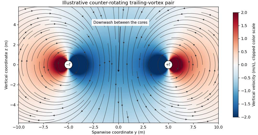
The wake is not generally two permanently straight tubes with fixed strength. A distributed trailing sheet rolls up, the cores move under induced velocities, and viscosity, turbulence and ambient motion alter the field. A wing’s actual span loading and operating state determine the wake, so the illustrative circulation and core size cannot be assigned to an aircraft merely from its visible span.
The connection to lift-induced drag is the complete induced-flow and load system. A short line sketched at each wingtip is not an extra independent friction force to add to an already complete drag calculation. The flow carries momentum and kinetic energy while changing the force direction experienced by the finite wing.
A proposed laboratory wake survey places a finite wing at a controlled load in a wind tunnel and measures transverse velocity at a downstream plane using calibrated directional probes or timed tracer images. Reverse the sign of lift to check the expected reversal of rotation, and compare measured circulation on several enclosing paths outside the cores. Tracers must follow the flow adequately, while finite sampling, tunnel walls and the probe’s own disturbance limit the inference. A visible tracer pattern alone does not supply the full three-dimensional velocity or pressure field.
The span efficiency factor compares a wing’s lift-induced drag with a reference induced-drag level at the same lift, span and dynamic pressure. In the conventional finite-wing coefficient model,It describes the induced contribution under stated geometry and flow assumptions. NASA’s primary account gives this relation and identifies the elliptic-load ideal in its lifting-line discussion.[ref]
For an ideal planar wing in classical lifting-line theory, elliptic span loading minimizes induced drag for fixed lift and span, corresponding to in this normalization. Deviations of the loading can increase induced drag and lower . The load distribution depends on twist, section properties and operating conditions as well as planform. An outline alone therefore does not specify a universal efficiency value. Nonplanar systems and different reference conventions require their own interpretation before applying the planar bound.
For an original coefficient example, choose , and . Then . With and , lift is and induced drag is about . At with those other quantities fixed, induced drag would be about . Thus the chosen corresponds to a 25-percent induced-drag increase over that reference, not a statement that twenty percent of all input power is lost.
A drag-polar fit illustrates why efficiency definitions can differ. Suppose a model haswhere is an additional lift-dependent profile-drag coefficient and is the induced efficiency. Fitting the entire quadratic term as givesFor stipulated , and , the fitted value is about . The algebra does not identify with the induced-only factor. It shows how a total-drag fit can absorb another modeled contribution even when the induced flow itself has not changed.
The inversion is also sensitive to a small extracted drag. At fixed and , a small fractional error in gives approximately the opposite fractional error in . If induced drag is obtained by subtracting a large estimated profile contribution from total drag, uncertainty in that subtraction can dominate. Different reference areas or lift conditions also change the comparison.
A proposed test combines measured lift and drag with a separately justified profile-drag estimate or a calibrated wake-based induced-drag inference. Repeat over the intended coefficient range and report the geometry, area convention, flow regime and uncertainty. A single fitted number is useful only alongside the model that separates induced drag from the rest of the measured aerodynamic force.
Elliptic span loading is a distribution of lift per unit span proportional to a half-ellipse, vanishing at both tips of a planar wing. For span and total lift , writeThe normalization follows by setting and using . It specifies a load distribution, rather than the wing outline. Classical lifting-line theory identifies this loading as the minimum-induced-drag solution for fixed total lift and span in its ideal planar setting.[ref]
Induced Drag Coefficient by NASA Glenn Research Center. Lifting Line Theory, elliptic distribution and efficiency normalization
The loading corresponds to circulation magnitude , with under the chosen positive-lift convention. Its ideal downwash at the lifting line is constant,Using dynamic pressure recovers and the span efficiency factor in that normalization.
A Fourier series makes the minimum transparent. In the classical lifting-line expansion, put andAt fixed and , is fixed and every higher-order contribution to drag is nonnegative. The minimum has only , yielding the half-ellipse. A higher-harmonic penalty in span loading quantifies departure from it: if is the only additional term, , so and induced drag rises three percent under the stated constraints.
For an original loading example, and give a central load . At it is of the central value. With and , the model gives , and .
A proposed test integrates measured surface pressure around several wing sections to estimate , then compares the normalized distribution and a wake survey with the model. An elliptic planform does not alone guarantee elliptic loading: section characteristics, incidence variation, deformation and operating conditions also enter. Nonplanar lifting systems, fixed bending-moment constraints and viscous or compressible effects change the optimization problem; the fixed-lift, fixed-span planar result should not be generalized beyond its assumptions.
A higher-harmonic penalty in span loading is the increase of ideal lift-induced drag caused by nonfundamental terms in a wing's circulation distribution at fixed total lift and span. In the classical planar lifting-line theory expansion, choose andHere is span, is freestream speed, and the coefficients are dimensionless. The primary force calculation uses this circulation expansion, the local lift law and sine orthogonality to obtain the lift and induced drag.[ref]
Force Calculations for Lifting Line (16.100) by MIT OpenCourseWare. printed pp. 1–3, circulation expansion and force integration
Because and , the integral for total lift selects only . The induced angle contains . Integrating its product with the loading then givesThe orthogonality identity behind both reductions isA higher harmonic can thus have zero net lift contribution while still adding positive induced drag. Its effect on local loading has not disappeared merely because its span integral vanishes.
For nonzero , division by the elliptic reference givesThe pure first harmonic gives elliptic span loading and . At a fixed relative coefficient magnitude, a larger order carries a larger penalty. Changing a coefficient's sign can redistribute the loading without changing its own squared contribution in this ideal model.
For an original example, take , and all other higher terms zero. The excess is , so . With and ,At and , the corresponding induced drags are about and . The higher harmonics add to this induced contribution, rather than to every source of aircraft drag.
A truncation error in an inferred span-efficiency factor matters when fitting sparse load measurements. Omitting nonzero terms makes the ideal-model drag sum too small at a fixed known , while fitting noisy high orders can inflate it because the terms are squared and weighted by order. If a justified bound is , then . A fit residual alone does not supply that bound.
A proposed experiment reconstructs section lift or circulation from a spanwise pressure survey, fits a declared set of modes, and compares the predicted induced contribution with an independent wake-based estimate. Report sampling density, load uncertainty and truncation choice. Viscosity, compressibility, nonplanar geometry or constraints other than fixed lift and span change the physical optimization problem; the quadratic penalty belongs to the stated lifting-line model.
Viscous drag is resistance to relative motion arising from viscosity. It transfers momentum between a moving object and its surrounding fluid, with mechanical energy dissipated as heat.
For a rigid sphere of radius moving at speed through an unbounded Newtonian fluid with dynamic viscosity , Stokes law gives drag magnitude in the creeping-flow limit. The force opposes relative motion. This linear law requires a small Reynolds number; a quadratic drag law appropriate to other flow regimes cannot be substituted without checking the assumptions.
Air resistance is drag produced by motion relative to air. It transfers momentum between the body and the air and can change both speed and trajectory. The relevant speed is relative to the local velocity field, so a wind changes the force even when the body's velocity relative to the ground is unchanged.
A quadratic model writes , with specified reference area . It is a regime-dependent representation, not a universal formula with constant . For a falling object under steady downward motion, terminal velocity occurs when the upward drag and any buoyancy balance the object's weight. Comparing differently shaped bodies of equal mass illustrates why neglecting air resistance can be accurate for one object and poor for another, even over the same fall distance.
Linear drag opposes the velocity relative to the surrounding medium with magnitude proportional to its speed, where . Its power is , so it dissipates kinetic energy. Under a constant external force, the resulting linear ordinary differential equation relaxes exponentially on the time scale .
For constant acceleration vector and , a projectile initially at with velocity hasThe integrating factor solves the first-order linear ordinary differential equation for the velocity; one more integration proves the position formula. The terminal velocity is , and is the relaxation time. For and , eliminating time when givesFor finite , the physical domain is . If , the path is vertical and cannot generally be represented as a single-valued graph . Expanding at fixed as recovers .
Mechanical mobility relates a steady drift velocity to a weak applied mechanical force. For isotropic linear drag , terminal force balance gives with , in units . For a sphere obeying Stokes's law, it is . The corresponding translational hydrodynamic mobility matrix is . The Stokes–Einstein relation reads , and the velocity relaxation time is . In the bare-force spherical model, a particle with electric charge has electrophoretic mobility ; ionic-atmosphere effects can modify that simple model.
When momentum relaxes much faster than the imposed motion, force balance replaces the inertial equation: in a deterministic one-dimensional model. The linear friction coefficient sets the time scale. Thermal forcing, if included, gives overdamped Langevin dynamics.
The dimensional linear friction coefficient relates drag force and velocity, , and has units of force divided by speed. It differs from the dimensionless aerodynamic drag coefficient. For an isolated sphere in Stokes flow, the Stokes drag law gives .
For constant downward gravitational acceleration and linear drag , the upward velocity solves with . Its first zero occurs at the displayed time. The dimensionless control variable is , and the limit gives .
The drag coefficient measures a drag force against a specified scale of force. Let be the body's velocity relative to the distant, undisturbed fluid, and let be its relative speed. For fluid density , drag force magnitude and reference area , defineThe drag coefficient is a dimensionless quantity: the denominator has units of force. The reference area must be reported with it. For a sphere of radius , the usual choice is the frontal area . Choosing its entire surface area instead divides the reported drag coefficient by four for the same physical drag force. Comparing coefficients without comparing their reference areas can therefore be misleading. [ref]
https://www1.grc.nasa.gov/beginners-guide-to-aeronautics/drag-coefficient/. NASA Glenn Research Center, Drag Coefficient, definition and Determining Value for Drag Coefficient
For a rigid sphere in steady flow through an unbounded Newtonian fluid with constant dynamic viscosity , incompressible flow and the no-slip boundary condition, the creeping-flow limit requires the diameter-based particle Reynolds number . The Stokes drag law gives . Substitution into the definition with gives the short derivationThus the drag coefficient is neither necessarily constant nor bounded above by one. The formula containing still describes linear drag here, because the drag coefficient varies as . The relation is the leading small-Reynolds number approximation, not a measured curve valid at every Reynolds number. [ref]
https://farside.ph.utexas.edu/teaching/336L/Fluid/node142.html. Richard Fitzpatrick, Axisymmetric Stokes Flow Around a Solid Sphere, equations 10.126 and 10.129
For a worked example, stipulate dynamic viscosity , density , radius and relative speed . Within the stated Stokes drag law assumptions,Doubling the relative speed with all other parameters fixed gives and : the predicted drag force doubles to . Falsely holding the drag coefficient at would instead quadruple the drag force. Both particle Reynolds numbers remain small, so the comparison is within the creeping-flow approximation.
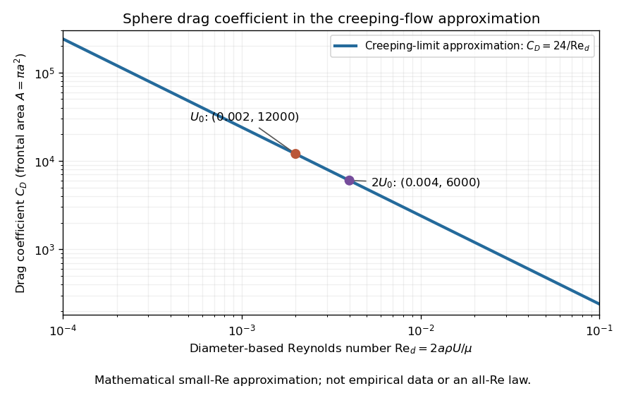
The useful idea is to separate the force scale from the dependence on geometry and flow conditions. A drag coefficient can help compare experiments, but changing Reynolds number can change the coefficient itself; NASA Glenn explicitly stresses matching the relevant flow conditions. The elegant cancellation above also exposes a common mistake: a drag coefficient definition does not by itself impose a quadratic drag law.
Quadratic drag has magnitude proportional to the square of the relative speed and points opposite to the relative velocity.
For an isotropic model of a body of fixed shape, let denote its relative velocity through the distant fluid, with . A constant positive resistance givesHere density , reference area and drag coefficient are held fixed over the modeled range of relative speeds. The vector formula makes the direction explicit: the drag force on the body opposes its motion relative to the fluid, and vanishes at . For a general body, orientation and other flow conditions can affect the drag coefficient; treating it as a constant requires a regime in which that is an adequate approximation. [ref]
https://www1.grc.nasa.gov/beginners-guide-to-aeronautics/drag-coefficient/. NASA Glenn Research Center, Drag Coefficient, Air Viscosity and Compressibility Effects
Compare two distinct models at a chosen relative speed . A linear drag model has , while a constant-coefficient quadratic drag model has . At their drag force ratios are two and four respectively.
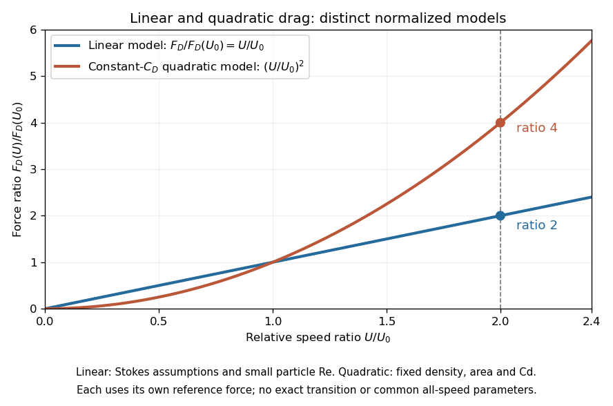
This distinction matters when estimating terminal velocity or trajectories such as descent from rest under quadratic drag: doubling relative speed increases the resistance much more strongly in the quadratic drag model. An approximately constant drag coefficient can occur in another Reynolds number regime; its use must be justified there. Conversely, substituting the creeping-flow sphere coefficient into recovers linear drag, so writing this general formula does not make the resistance quadratic. Neither approximation should be extended across all Reynolds numbers.
The distinction already appears in the original investigation underlying the Stokes drag law, read on 9 December 1850: article 42 identifies resistance proportional to relative speed and distinguishes it from a contribution proportional to the square of relative speed. [ref]
Let downward velocity obey , with constants , terminal velocity and initial speed . Gravity minus buoyancy can supply the constant downward force represented by . Since , the equation for is linear in depth: , giving the displayed decay. Exact terminal velocity is approached only asymptotically. A practical tolerance is attained at , provided the initial excess exceeds that tolerance. Its time-domain form is with , in contrast to the hyperbolic tangent for descent from rest under quadratic drag.
For positive downward speed, gravity and quadratic drag give , . Separation and the integral of give the displayed approach to terminal velocity. The fallen distance is . The limit as recovers and distance .
For an ice mass in still water, approximate the wind stress by a fixed vector while retaining quadratic drag in the water. With mass per water-drag area , water coefficient and , the steady balance is . Resolving along the drift and perpendicular to it gives , . Thus and . The direction is right of the wind in the northern hemisphere and left in the southern hemisphere. This angle neglects intrinsic boundary-layer turning, ocean currents and contact forces; it is not a universal observed sea-ice turning angle.
The normalization has units . It converts the Coriolis force into a force per water-drag area and allows comparison with wind and water stresses. Icebergs generally have much larger than thin ice floes, but their effective air-to-water drag-area ratio also matters. A geometric depth becomes a mass per area only after multiplication by density.
A resistive velocity term proportional to the speed squared removes energy at rate proportional to . Its derivative at zero velocity vanishes, so it does not appear in the linearization of a dynamical system at rest. Nonlinear energy arguments can still prove asymptotic stability.
Pressure drag is the component of force produced by integrating pressure over a body's surface. For flow over topography , the horizontal force on the fluid is to leading order.
The Stokes number compares a particle's drag stopping time with a characteristic flow time : . In an orbiting disk, the natural choice is .
Gas drag is a drag force on a solid body due to its motion relative to surrounding gas. With aerodynamic stopping time , the linear approximation gives .
The aerodynamic stopping time is the characteristic time on which drag force damps a solid particle's velocity relative to the surrounding fluid. Linear drag gives relative acceleration .
A potential flow has a velocity field represented by a scalar velocity potential, . Its vorticity vanishes wherever is sufficiently smooth. In a constant-density incompressible flow, mass conservation additionally gives Laplace's equation .
This reduces a vector-flow problem to a scalar boundary value problem. Linear combinations of elementary source and sink potentials can construct flows around simple geometries. The representation can be local even when a globally single-valued potential fails: a circulation-carrying flow around an excluded core has zero vorticity in the fluid region but can have nonzero circulation around the hole. Neglect of viscous effects also limits predictions near solid surfaces and in a wake. A useful potential-flow approximation therefore needs both its domain and its treatment of boundaries stated explicitly.
A uniform planar stream combined with an equal source and sink produces a closed dividing streamline enclosing them. Outside it the flow approaches the uniform stream; inside it streamlines connect the source and sink. For positive and separation one, the complex velocity is and the stagnation points are . Both lie on the dividing streamline, which has zero streamfunction with consistent logarithm branches.
The Kutta condition selects the circulation of an idealized potential flow past a body with a sharp trailing edge by requiring finite limiting velocity at that edge. For the Joukowski map , the trailing edge corresponds to a simple zero of at . If is the complex potential in the circle plane, then is finite there only if . For a uniform flow of speed at angle and a point vortex of circulation , this gives , and cancellation of the simple zeros gives the tangential trailing-edge velocity . The opposite endpoint can retain a leading-edge singularity.
For , the Joukowski map maps the exterior unit circle to an ellipse of horizontal and vertical semiaxes and . The Milne-Thomson circle theorem gives for a uniform flow inclined by . The chain rule produces the displayed complex velocity in the physical plane. Since , the far-field flow retains its speed and direction. Its two stagnation points areobtained from . The map derivative is nonzero on and outside the unit circle, so these zeros are preserved without introducing a boundary singularity.
For a smooth constant-density exterior potential flow satisfying the finite-energy condition for planar exterior potential flow, use and the planar streamfunction convention , . Since , . Apply the divergence theorem to a truncated exterior region. The outer term vanishes; on a counterclockwise body boundary the body's outward normal satisfies , while the fluid's outward normal points the opposite way. This gives the displayed kinetic energy per unit span. The formula yields the added mass of a circular cylinder directly from its surface values of and .
For a planar potential flow outside a bounded body, suppose its single-valued complex velocity is holomorphic near infinity and tends to zero. Its exterior Laurent series begins . The outward volume flux and counterclockwise circulation satisfy . Thus both vanish precisely when the leading term is absent. A nonzero gives and logarithmically divergent exterior kinetic energy. When , and the far-field energy integral converges. Zero circulation alone does not exclude the radial source field .
For a fixed impermeable sphere of radius and incident uniform flow , the velocity potential is the displayed expression and the Stokes streamfunction is . Differentiation gives and . Thus the no-penetration boundary condition holds, the poles are stagnation points, and the equatorial surface speed is . The disturbance is a potential dipole decaying as in velocity. The sphere theorem for a Stokes streamfunction constructs this solution from .
For a sphere translating through an unbounded inviscid incompressible fluid at rest far away, the laboratory fluid velocity written in coordinates centred on the moving sphere is the gradient of the displayed dipole potential. Its radial velocity at the surface equals . The sphere-rest-frame velocity instead needs the additional uniform potential .
For an incompressible irrotational two-dimensional potential flow, an analytic complex potential of a two-dimensional potential flow combines the velocity potential and streamfunction . The Cauchy-Riemann equations give and , hence . Curves of constant are streamlines. An analytic coordinate change transforms the complex velocity by wherever .
A planar potential dipole at with complex moment has complex potential of a two-dimensional potential flow . Its complex velocity is , interpreted as . Unlike the three-dimensional potential dipole, this is a two-dimensional singularity of the logarithmic-source potential. For example, two opposite source coefficients at have potential , whose leading term is as the separation tends to zero with fixed. This gives the dipole as a limiting source–sink pair, with the complex sign and orientation included in .
A transported planar potential dipole follows the surrounding regular velocity, so its position satisfies the displayed equation after its own singular term is removed. The conjugation comes from the convention . Reflected image parameters are held fixed when taking the spatial derivative, then evaluated at the instantaneous dipole position.
For a unit circular wall, the Milne-Thomson circle theorem gives image potential and therefore . For a horizontal straight wall the image is , giving . For the line , reflected conjugation gives image and hence . In each case the image lies outside the fluid region and makes the wall a streamline; differentiation of the regular image proves the motion formula. Several compatible straight-wall reflections can be summed before the same operation is applied.
For a complex potential , reflection in the straight wall through zero at angle is . The image construction givesOn the wall , this is real, so its stream function is constant there. This proves the impermeability condition. Thus the image position is and its moment is . If the point dipole is advected by the regular image flow, the complex velocity convention giveswhere is its signed distance from the wall. The last equality follows from . It applies when .
A two-dimensional point sink of strength removes volume flux per unit depth at . Its complex potential of a two-dimensional potential flow is the displayed expression, so . The radial velocity is : integrating over a circle gives outward flux . This is the planar cross-section of a line sink. A passive particle satisfies and reaches the ideal point singularity in finite time. This is a flow singularity, distinct from a stable sink equilibrium of a regular dynamical system.
For a two-dimensional potential doublet of fixed complex strength outside a stationary circle of radius , the Milne-Thomson circle theorem gives the image contribution . If the singularity is stipulated to follow the regular fluid velocity at its position, differentiating this term and using the complex velocity convention gives the displayed motion law. Thus is constant: the trajectory is a straight line parallel to . With and initial location real, its polar coordinates satisfy . This statement assumes fixed orientation; the translational rule alone supplies no equation for orientation evolution.
For a steady two-dimensional incompressible flow and irrotational flow around an impermeable body, the displayed contour formula gives the force on the body per unit span. Here is the complex velocity, is the constant mass density, and runs counterclockwise around the body, excluding other fluid singularities. To verify the sign, Bernoulli's principle gives . On a counterclockwise boundary, the complex pressure force is . Tangency gives , and therefore . Integrating removes the constant term and gives the formula. The theorem is named after Heinrich Blasius.
The Milne-Thomson circle theorem places an image dipole inside a cylinder at the inverse point of an external dipole. In the residue of the squared complex velocity, only the cross term between the analytic external velocity and the image double pole contributes. The product of their conjugate dipole strengths is independent of orientation, so the cylinder force is radial toward the external dipole.
For a two-dimensional steady ideal flow outside a body, let be the complex velocity. Suppose is holomorphic in the exterior and has a Laurent series near infinity, with coefficient of . Orient the body contour counterclockwise and assume the usual impermeability and Bernoulli hypotheses of the Blasius force theorem. Deforming the contour to a large circle gives . Substitution in Blasius' formula proves .
In particular, makes the force zero: its square has no reciprocal term. This criterion handles branch-cut obstacles by applying the contour in their analytic exterior, rather than separately assigning forces to endpoint singularities.
Place a held point vortex of circulation at real position outside a circular cylinder , and prescribe circulation about the cylinder. An opposite image at gives complex velocity . On the positively oriented cylinder contour, the only pole of inside is at , with residue . The residue theorem and Blasius force theorem give . Thus and : the force on the cylinder points toward the vortex. The specified cylinder circulation is part of the hypothesis; a zero-circulation cylinder has an additional central image term.
For steady incompressible flow and irrotational flow of constant mass density, with no body force, this formula gives the hydrodynamic torque about the origin per unit span on an impermeable body. Orient its boundary counterclockwise, and let positive torque be counterclockwise. The proof uses , the Bernoulli equation , and the tangency identity . The real part of the constant-pressure term vanishes because . The full complex integral of need not vanish.
In a planar potential flow, superpose a positive- uniform flow of speed and a line source of strength at the real point . Introduce an impermeable unit circular cylinder with zero circulation. The Milne-Thomson circle theorem gives the complex potential of a two-dimensional potential flowThe displayed horizontal force per unit length acts on the cylinder, and by reflection symmetry. To prove it, let be the complex velocity. At infinity, , so the sum of all finite residues of is . At the external pole , write ; thenThe residue theorem and the counterclockwise Blasius force theorem give , proving the formula. With and , its sign changes at .
The Milne-Thomson circle theorem constructs a circular impermeable boundary in a two-dimensional potential flow. Suppose an incident complex potential of a two-dimensional potential flow is analytic on and inside , with its physical singularities outside that disk. Then the displayed has constant stream function on . The proof is the identity on the circle: there is real. Hence the circle is a streamline and satisfies the no-penetration boundary condition. The reflected term has its image singularities inside the obstacle. Additional imposed circulation must be specified separately. The theorem is named after Louis Melville Milne-Thomson.
Articles were limited to the first 100 out of 176 total.
Articles by others on the same topic

Fluid dynamics is a branch of physics and engineering that studies the behavior of fluids (liquids and gases) in motion. It involves understanding the forces and interactions that govern the flow of fluids, how they move, and how they interact with solid boundaries and other fluids. Fluid dynamics is governed by the principles of fluid mechanics, which encompass both fluid statics (the study of fluids at rest) and fluid dynamics (the study of fluids in motion).