The Lorentz force is the force exerted by an electric field and a magnetic field on a body with electric charge and velocity . In SI units its form in nonrelativistic classical mechanics, using mass and Newton's second law, isBoth fields are evaluated at the body's position at the current time. The electric field contributes even at rest, whereas the magnetic force depends on velocity through a cross product. [ref]
https://openstax.org/books/university-physics-volume-2/pages/5-4-electric-field. OpenStax, electric force and field
; [ref]https://openstax.org/books/university-physics-volume-2/pages/11-2-magnetic-fields-and-lines. OpenStax, magnetic force on moving charge
.For a concrete charged particle in a uniform magnetic field, use nondimensionalization to stipulate , magnetic field , zero electric field, initial position , and initial velocity . These are rescaled quantities, not an assertion that the mass, electric charge, and magnetic field have the same physical units. At the start, , so the magnetic acceleration points toward . The resulting circular motion isAt the position is and the velocity is ; at the position is and the velocity is . Thus the circle has center and radius one. Viewed from toward the plane, the motion is clockwise. Changing only the electric charge to gives position and reverses the bending to counterclockwise.
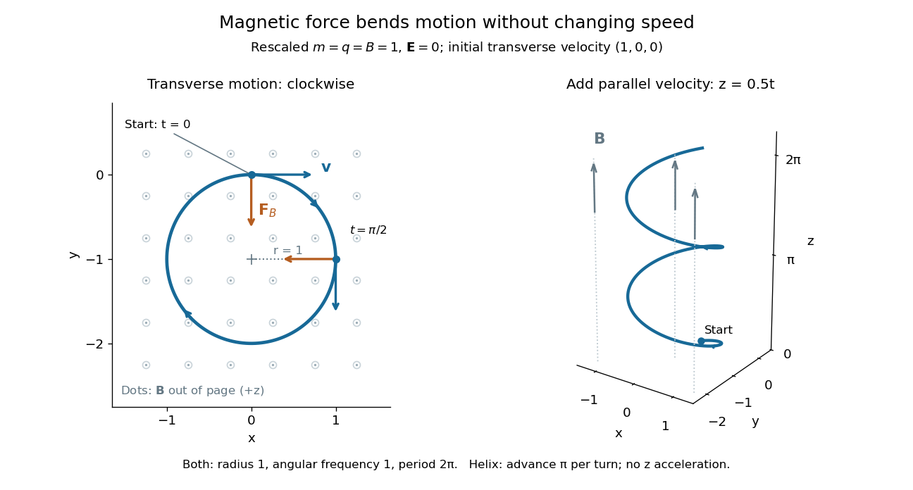
Adding initial velocity leaves the transverse circular motion unchanged and givesThis is a helix of transverse radius one, cyclotron frequency , and transverse period ; the advance along in one turn is . The parallel component of velocity stays constant because the magnetic force has no parallel component: there is no magnetic acceleration along the magnetic field. If the initial velocity were entirely parallel to the magnetic field, the magnetic force would vanish and the path would be straight. [ref].
More generally, with zero electric field, no other forces, and a uniform constant magnetic field of magnitude , decompose velocity into perpendicular and parallel components. For nonzero electric charge , the perpendicular speed determines the gyroradius, while the cyclotron frequency is an angular frequency:These are nonrelativistic formulas; see the relativistic cyclotron orbit for the correction. The beauty is that increasing perpendicular speed increases the radius in exactly the proportion needed to leave the period unchanged. Conversely, known magnetic field, perpendicular speed, and measured radius determine the magnitude of the electric charge divided by mass. This makes the same geometry useful for comparing bodies with different electric charge and mass.
Two short checks explain the result. First, the cross product gives for both stipulated positive-electric charge paths, exactly their acceleration. Second, the transverse magnetic force supplies the centripetal acceleration, so ; for this gives the gyroradius, and gives the cyclotron frequency.
Magnetic forces do no work: the instantaneous power of the magnetic part of the Lorentz force vanishes because a cross product is perpendicular to its first argument. The work-energy theorem therefore givesThe dot product is zero at every instant, rather than only after a full turn. With zero electric field and no other forces, the kinetic energy and speed remain constant; the electric field can increase or decrease kinetic energy according to the sign of . In the two stipulated examples the constant kinetic energy is respectively and in rescaled units. The extra parallel velocity raises kinetic energy without changing the gyroradius or the cyclotron frequency.
For an electric example in rescaled units, stipulate , zero magnetic field, constant electric field , no other forces, and rest at . The Lorentz force gives acceleration and velocity , hence kinetic energy and power . At , the kinetic energy has risen from zero to two: the electric field has done positive work.
The existing electromagnetic field tensor formulation expresses the same interaction covariantly. For four-momentum and four-velocity , using proper time , the Lorentz force law isIts spatial and temporal components are
A nonrelativistic charged particle entering a uniform magnetic region normally at one plane follows a circle of radius . If the field extends through a normal thickness , the particle enters the strict region beyond the far plane only for . Equality gives tangency, not crossing. For transmission, its deflection angle obeys . The result assumes a sharp field boundary, fixed speed in the magnetic region and no electric field there.
Rapid circular particle motion perpendicular to a locally uniform magnetic field, superposed on parallel streaming when the parallel velocity is nonzero. In Gaussian units, its signed cyclotron frequency is given in the title and its gyroradius is . Slowly varying fields permit a guiding center description.
For a constant perpendicular force in a uniform magnetic field, write the particle velocity as . Choosing leaves the ordinary gyromotion equation for . The gyroperiod-averaged transverse velocity is therefore the displayed drift. An electric force gives the same drift for both charge signs; a charge-independent applied force gives opposite drifts.
For a curved field direction , define the curvature vector . Motion along curved field lines produces a gyroaveraged drift perpendicular to both field and curvature. In a purely toroidal field this and magnetic gradient drift cause opposite vertical drifts for opposite charge signs.
A slowly varying field magnitude exerts the gyroaveraged force on a particle with magnetic moment . Applying the perpendicular-force guiding-centre drift formula gives the displayed velocity. Its direction depends on the sign of the particle charge.
The magnetic contribution to the Lorentz force on a point charge. It is perpendicular to that charge's instantaneous velocity, so its direct work on the charge is zero. Summing contributions in a conductor leads to the magnetic force on a current-carrying wire; mechanical work in moving circuits must also account for the electric fields and constraints that maintain the current.
For a square spanning , with current counterclockwise as seen from positive , an applied field vanishes on two edges. Integrating on the other two gives the displayed force. Its direction reverses with the current. The formula concerns the loop, not unspecified supply leads, and cannot be replaced by a small-loop approximation without checking the field variation.
The radius of a charged particle orbit perpendicular to a uniform magnetic field. In a parabolic band , or for a Fermi-level electron. Charge sign sets the curvature direction, while the radius uses magnitudes.
Magnetic rigidity measures the resistance of a charged particle's momentum to bending by a magnetic field. The relativistic cyclotron orbit gives , where is the transverse gyroradius. For motion perpendicular to a uniform magnetic field, is the whole momentum. A measured magnetic rigidity fixes momentum per magnitude of electric charge; it does not by itself fix mass, kinetic energy, or the sign of the electric charge. This distinction makes the Anderson positron track experiment an especially revealing application of the Lorentz force.
The Anderson positron track experiment identified a light positively charged particle, now called the Positron, by combining magnetic bending, loss of kinetic energy in lead, and particle range. Each observation answered a different question: bending constrained momentum, the lead supplied a direction of travel, and particle range tested the proposed mass.
Carl David Anderson's The Positive Electron (1933), pp. 491–493, describes the 1932 discovery in a vertical cloud chamber with a magnetic field. A lead plate separated two photographed track segments. The effective viewing depth was along the magnetic field, with transverse diameter: this restricted out-of-plane motion. The photographic readout supplied curvature on both sides. Comparisons with electron tracks under the same conditions constrained ionization; specific ionization was not directly measured for these events. He tested accidental alignment of unrelated tracks and rejected a reversed electron interpretation requiring an increase of kinetic energy in lead. Assuming unit electric charge, the mass bound was about twenty electron masses, rather than an exact mass determination. The paper credits Robert Andrews Millikan with the design and Seth Henry Neddermeyer with assistance.[ref]
The Positive Electron by Carl David Anderson. pp. 491–493, Fig. 1 and charge/mass discussion; p. 494, acknowledgment
Preparation used rapid piston expansion and a water–alcohol mixture in the cloud chamber; cooling permitted droplets to form along ionization trails. A camera photographed these droplets. Initially, expansions occurred at random, so many photographs contained no tracks. Later counter triggering improved the useful yield.[ref]
Carl David Anderson by William Hayward Pickering. Biographical Memoirs: Volume 73; William H. Pickering, Carl David Anderson, pp. 27–28: preparation, photographs and timing
In The Production and Properties of Positrons, his 1936 lecture, Carl David Anderson describes the chamber inside an electromagnet and explains why the lead plate was decisive: after losing kinetic energy, a particle bent more sharply. He describes a proton hypothesis predicting only of particle range, against an observed path longer than . These are historical values from the lecture, not the stipulated example below. The point was the incompatibility of particle range with the momentum inferred from curvature, rather than positive electric charge alone.[ref]
The Production and Properties of Positrons by Carl David Anderson. Nobel Lectures, Physics 1922–1941; pp. 365–366, electromagnet, lead-plate direction test and proton range comparison
A photograph records a path but supplies no arrow of time. The Lorentz force depends on : reversing both electric charge and direction of travel leaves the spatial bending compatible with the same path. Thus a particular arc can represent a Positron travelling one way or an electron travelling the other. Knowing the magnetic field's polarity is necessary but insufficient. Gravity does not justify assuming that every cosmic ray track travels downward.
The lead plate adds a physical ordering. For a single particle crossing a passive absorber without an accelerating interaction, the outgoing momentum is smaller, so the outgoing gyroradius is smaller in the same magnetic field. The less curved segment comes first. Once this direction is assigned, the cross product in the Lorentz force determines the sign of electric charge. For the convention below, points out of the page; at upward velocity , . Bending to the right therefore means positive electric charge.
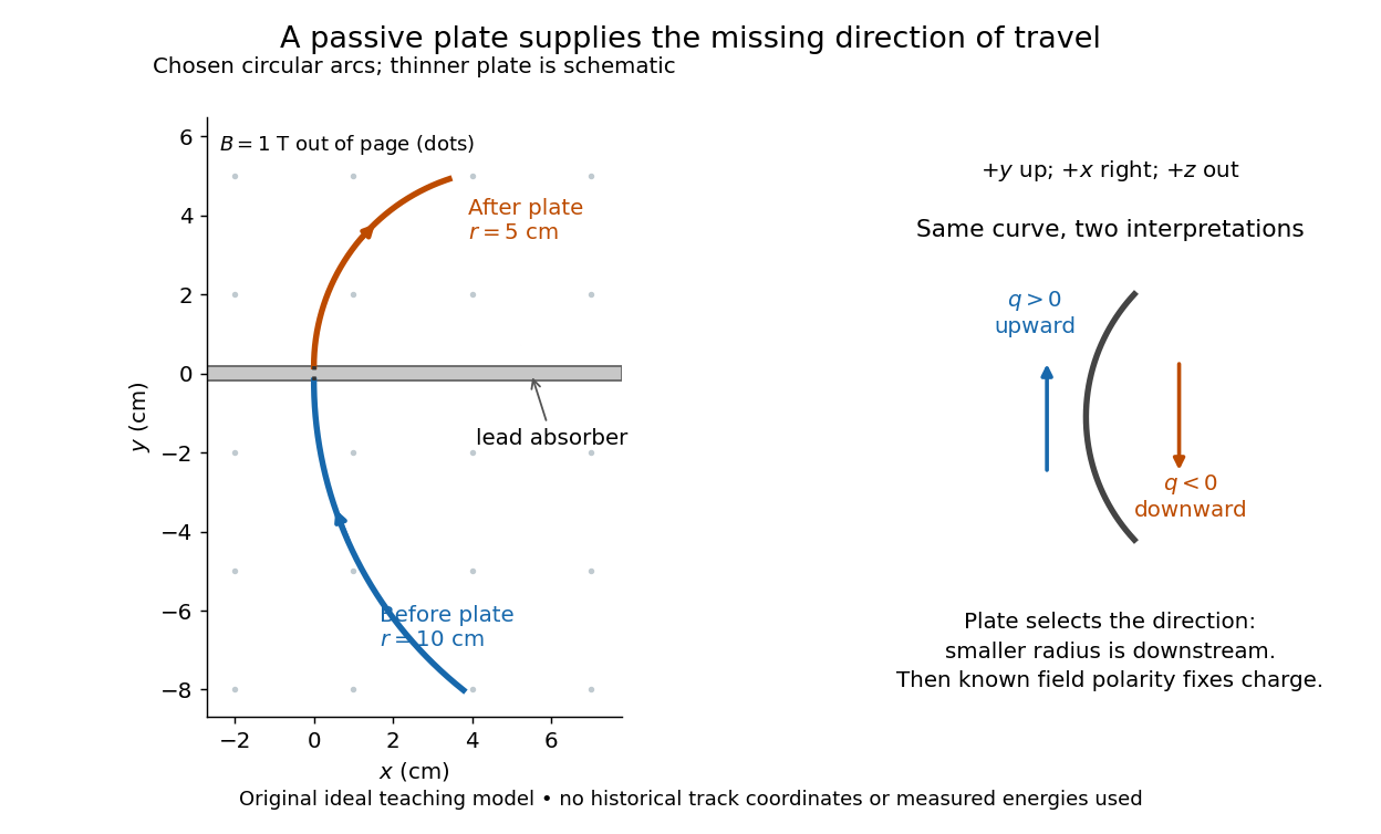
Magnetic forces do no work: the change of kinetic energy occurs through interaction with the material, not through the bending magnetic field. The ideal construction suppresses multiple scattering, kinetic energy fluctuations, and loss of kinetic energy in the gas. In an actual analysis one compares arcs away from the plate and allows a change of tangent from multiple scattering; one cannot interpret every kink as a change of electric charge. Short visible arcs, uncertain projection and small bending also limit a determination of magnetic rigidity.
For a concrete independent example, stipulate perpendicular motion, with the elementary charge, uniform magnetic field , incoming gyroradius and outgoing gyroradius . These are invented teaching inputs. Converting SI momentum to electronvolt units givesso and . Both a Positron and a proton with these momenta trace the same ideal arcs. Their kinetic energies differ because the relativistic energy-momentum relation givesThe second expression avoids subtracting nearly equal quantities when . For this calculation stipulate rounded rest energies and . The Positron interpretation gives and ; the proton interpretation gives only and . The corresponding proposed losses of kinetic energy are about and .
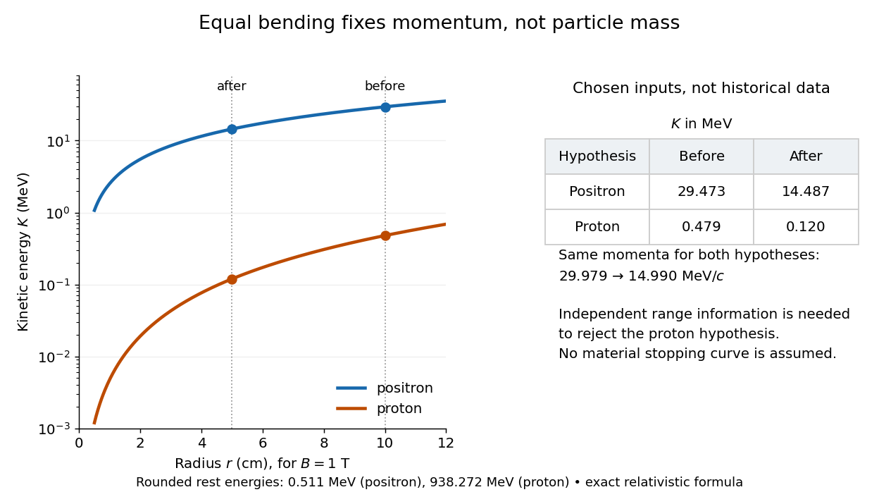
The small proton kinetic energy follows from , whereas here the Positron has and . Consequently magnetic bending alone cannot reject the proton. One needs an independent material constraint: could a proton at the proposed kinetic energy penetrate the plate and then travel at least the observed visible distance in the specified gas? A particle range shorter than that visible distance contradicts the hypothesis. The visible track need not include the stopping point: it already supplies a lower bound on particle range. No numerical particle range is assigned to this teaching example; that would require stopping data for the actual material and gas conditions. The experimental insight is to combine a geometric momentum measurement with an independent test of penetration.
The charge-to-mass ratio is a body's electric charge divided by its mass . Its SI unit is the coulomb per kilogram, . In a prescribed electric field and magnetic field, nonrelativistic acceleration depends on through the Lorentz force. Two bodies with the same initial position, velocity, and charge-to-mass ratio therefore have the same trajectory in this ideal model. For an electron, write with the elementary charge: , whereas the positive number is the magnitude of the charge-to-mass ratio.
A velocity selector uses perpendicular electric field and magnetic field to transmit a narrow range of speeds along a chosen beam direction. Assume uniform static electric field and magnetic field , with , and an incident velocity . The cross product gives , so the transverse Lorentz force isFor an electron, the electric force points downward and the magnetic force upward. A faster electron initially bends upward; a slower one initially bends downward. At the selected speed, both forces cancel along the whole straight trajectory. The cancellation is independent of mass and nonzero electric charge; it selects velocity, not a particular charge-to-mass ratio. A component of velocity parallel to the magnetic field is not constrained by the cancellation, so the incident beam must also have its direction restricted.
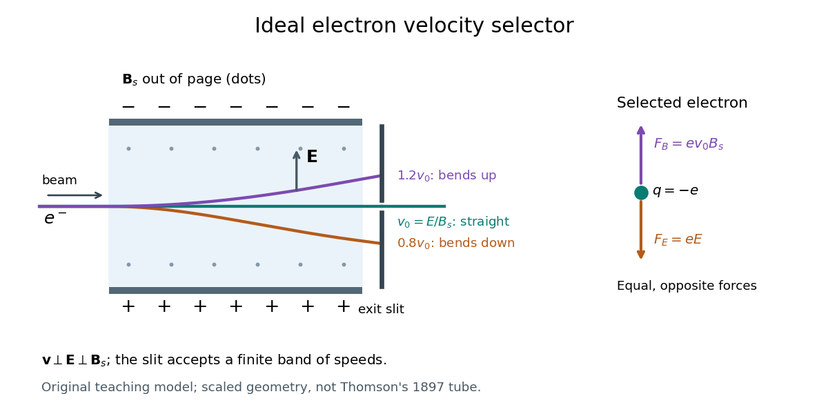
A real exit slit accepts a finite range of speeds and incident directions. A zero displacement at one screen alone does not establish zero force throughout the path: a curved trajectory could return to that screen position. The ideal velocity selector interpretation requires a straight aligned beam, known overlapping electric field and magnetic field, and sufficiently narrow entrance and exit slits. Its useful role in the Thomson charge-to-mass experiment teaching model is to supply speed independently of the subsequent magnetic bending.
The Thomson charge-to-mass experiment infers the magnitude of an electron's charge-to-mass ratio by combining electric and magnetic deflection of cathode rays. The central idea is to determine speed separately from magnetic curvature: a known speed turns the observed gyroradius into a measurement of .
In 1897, J. J. Thomson used two grounded slits in an evacuated glass tube, then aluminium plates long, wide and apart. A battery supplied their electric potential difference. Deflected cathode rays produced a phosphorescence patch on the glass; an external scale and movable luminous pointer recorded its position in darkness. Greater evacuation reduced gas electrical conductivity that screened the electric field; reversing plate polarity reversed deflection. External coils supplied the magnetic field, calibrated by induction against larger coils. He adjusted equal electric and magnetic deflections. [ref]
Cathode Rays by Joseph John Thomson. Cathode Rays (1897), Fig. 2; second m/e method, apparatus and calibration
His comparison included air, hydrogen, carbon dioxide, and aluminium versus platinum cathodes, supporting a common carrier. He explicitly noted uncorrected magnetic bending outside the plates. His tables give , the reciprocal of the magnitude used here. The inferred ratio alone could not separate electric charge from mass. [ref]
Cathode Rays by Joseph John Thomson. Cathode Rays (1897), second m/e method: table, corrections and interpretation
To connect this readout with the Lorentz force, derive a simple nonrelativistic model in modern SI notation. Let the uniform deflecting region have length , followed by a field-free drift of length . Assume a narrow speed distribution, small deflection angles, negligible collisions, and matching electric and magnetic field profiles. For an electron with speed , the electric acceleration has magnitude , the transit time is approximately , and the subsequent drift adds exit transverse velocity times . Thus the displacement magnitudes measured separately with only electric field or only magnetic field areThe electric expression follows from constant transverse acceleration; the magnetic expression uses its small-deflection approximation. Equal displacement magnitudes then giveThis is an ideal derivation of the comparison principle, not a numerical reanalysis of the historical tube. Different exterior magnetic field profiles invalidate cancellation of the common geometrical factor. The comparison determines through deflection and the known apparatus dimensions; it does not require a downstream semicircle.
For a second, deliberately different teaching geometry, combine a velocity selector with a separate region containing only a uniform magnetic field perpendicular to the selected velocity. Here belongs to the velocity selector, while belongs to the analyzer: they need not be equal. The magnetic Lorentz force supplies the centripetal acceleration, soIf the analyzer turns the beam through a semicircle before it hits a screen in the entry plane, the separation between entrance and impact is the diameter: . For a shorter observed arc, the screen displacement is not generally a radius; fit the appropriate circle geometry. This two-stage velocity selector and curvature apparatus is an original ideal teaching model, not a claim that Thomson's Fig. 2 used a separate selector and semicircular analyzer.
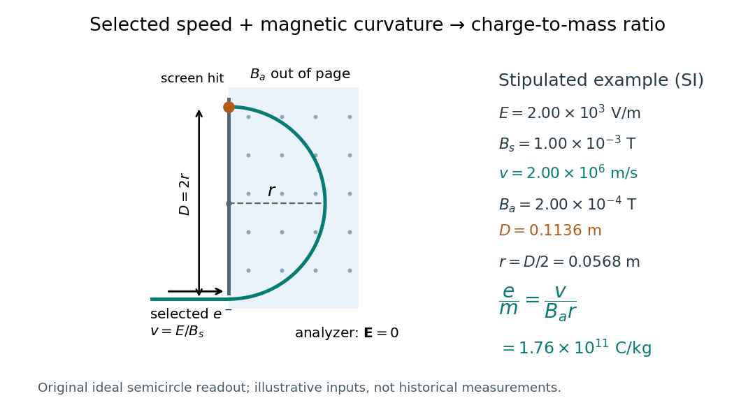
For a worked example, stipulate , , , and . The selected speed and inferred charge-to-mass ratio magnitude areThe SI units provide an independent check: and , because . The charge-to-mass ratio of the electron is negative; this calculation gives its magnitude. The bending direction gives the sign of the electric charge once the magnetic field direction is known. Scaling both and by the same positive factor preserves every displayed trajectory, so an independent electric charge measurement is required to determine mass separately.
The curvature formula assumes nonrelativistic momentum . At higher speeds, the relativistic cyclotron orbit gives , hence , where is the Lorentz factor; the ideal straight-through selection still follows from vanishing Lorentz force. The stipulated speed is about times the speed of light, making about . For this example the nonrelativistic approximation is adequate, but no massive particle can be selected at . Finite slit widths, collisions with residual gas, uncertain magnetic field calibration, and fields outside the ideal boundaries limit a real inference; repeat at several selected speeds and analyzer strengths to test consistency of rather than trusting one spot position.
The Lenard cathode-ray window experiment lets cathode rays leave a gas-discharge tube through a thin aluminium foil while preserving the tube's vacuum. This separates production from propagation.
Philipp Lenard's lecture, delivered on 28 May 1906, describes sealing a small hole in a metal plate with aluminium foil. Luminous phosphor grains first rested on the window, then glowed above it in air. His improved tube separated production and observation chambers; coated paper served as a fluorescent screen. An aperture revealed spreading beyond a narrow straight beam. Evacuating the observation chamber reduced spreading and attenuation without interrupting production. Interposed layers and stepped foil stacks gave shadow comparisons; approximate scaling with mass had exceptions.[ref]
On Cathode Rays by Philipp Lenard. On cathode rays, title page p. 105; pp. 108–114, Figs. 3–8: foil window, phosphor readout, aperture, layer comparisons and evacuated observation chamber
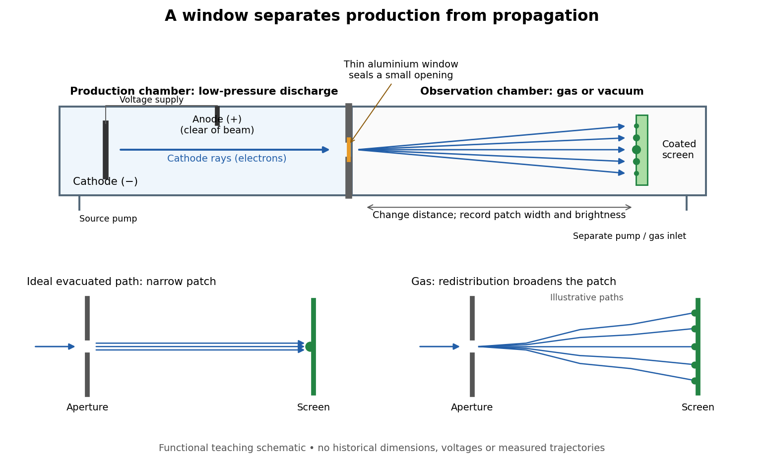
The experimental advantage is unusually clean: reducing the gas content in the observation chamber tests whether gas is needed to carry the cathode rays, while retaining the conditions needed to generate them. The window is a boundary that transmits some electrons while confining the source environment. A spot outside establishes a transmitted effect; the aperture and changed observation environment provide additional ways to distinguish propagation from the source's behavior. This logic is useful whenever a complicated source would otherwise be changed by the very intervention intended to test the emitted beam.
Several inferences require care. A darker fluorescent screen can mean fewer arriving electrons, less deposited energy per electron, or redistribution by electron scattering beyond the observed area. A visible endpoint depends on the screen's sensitivity and background. It is not an intrinsic electron range independent of initial kinetic energy, gas density, and observation geometry. For a modern comparison, measure a reference at fixed source conditions, use background subtraction, and compare the whole luminous patch as well as a small central region. A wider collection area tests redistribution; changing source-to-screen separation also changes collection geometry. These are proposed controls for interpreting a readout, not additional historical observations attributed to Lenard.
Nor is fluorescence a unique signature of cathode rays: X-rays can also excite it. Lenard notes that a later tube could transmit both, and that slow cathode rays failed to pass its window.[ref]
On Cathode Rays by Philipp Lenard. On cathode rays, pp. 114–115 and 120–121: X-rays in the later tube; limited transmitted velocity range
In modern terms, cathode rays are electrons carrying negative electric charge, whereas X-rays are photons with zero electric charge. Magnetic bending of the incident electrons, interpreted through the Lorentz force, supplies a discrimination that brightness alone cannot. Passage through foil alone determines neither the sign of electric charge nor its magnitude, and it does not measure charge-to-mass ratio. The separate Thomson charge-to-mass experiment explains that inference. Even a measured charge-to-mass ratio needs an independent electric charge measurement to determine mass.An original toy model separates two ways to lose a central cathode ray signal. Let be forward depth into a uniform gas. Normalize the entering electron population to one. Write for the fraction still in a narrow forward channel, and for the fraction diverted into a wider collection channel. Assume constant removal rate per unit depth in both channels, and constant transfer rate from to , with no return. Removal means that an electron stops or is trapped before reaching the collecting plane; it does not mean that its electric charge disappears. The wide ideal collector accepts all surviving members of both channels. This is a stipulated two-population differential equation model, not a general law of electron transport:The first equation gives exponential decay. Adding the equations gives for , henceThese formulas also give a conservation check: . The fraction has been removed before the plane, while remains present but misses the narrow collector. An exponential fit to the narrow signal therefore measures , not the removal rate by itself. This is an identifiability issue: one declining signal cannot distinguish the two unknown rates.
For a worked example, choose and . These are invented teaching inputs, not measured coefficients for air or Lenard's apparatus. At ,Thus about misses the narrow collector, although only about has been removed in this model. Treating the whole narrow-signal deficit as stopping would confuse redistribution with removal.
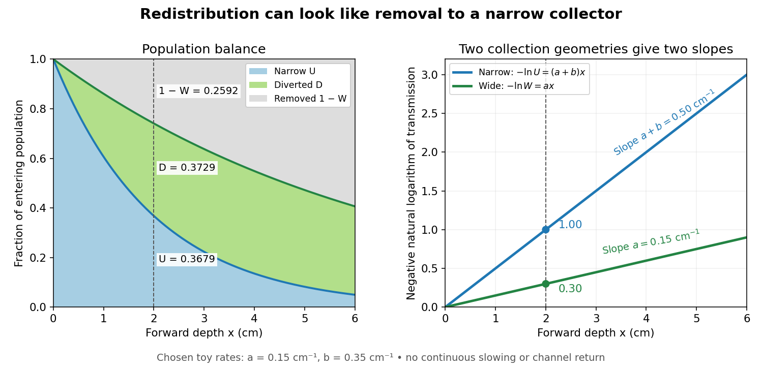
Suppose a calibrated readout is proportional to arriving electron number with the same response for either channel. Choose an empty-path signal arbitrary units, of which is background; the two collection geometries have the same calibrated reference. The calculated readings at are and . After background subtraction, define for each geometry. Then the original inverse problem has the solutionA single narrow reading would instead allow every nonnegative pair with . Using the raw ratios without subtracting gives an erroneous narrow rate of about . In a real fluorescent screen, the assumed response must be tested: deposited energy and conversion to light need not remain constant as electrons slow. Repeating the comparison at several depths tests the constant slopes, although straight slopes alone do not establish the microscopic mechanism.
Actual electrons change kinetic energy and direction. Electron stopping power describes mean kinetic energy loss per travelled path length ; collisional losses include ionization, while radiative losses include bremsstrahlung. The continuous slowing-down approximation range integrates reciprocal total electron stopping power, neglecting fluctuations. It approximates travelled path length, not forward penetration depth.[ref]
Appendix: Significance of Calculated Quantities. Stopping-Power and Range Tables for Electrons, Protons, and Helium Ions by M. J. Berger and others; Appendix: Significance of Calculated Quantities, collision/radiative/total stopping power, CSDA range, projected range and detour factor
As a separate original limiting example, stipulate a straight path, constant , and entering kinetic energy . Then until stopping, and . In that deterministic model every entering electron reaches each depth below and none crosses a plane beyond it. There is no exponential population tail. Real fluctuations and electron scattering make the situation more complicated, but the example already proves that continuous energy loss does not imply constant-rate removal.The window also changes the entering population: source kinetic energy before the foil need not equal just outside it. For an electron initially at rest, an ideal static accelerating electric potential difference supplies electrical work , where is the elementary charge. If losses before and within the foil total , a transmitted electron enters the observation chamber with . A screen's brightness determines neither nor . These formulas specify a modern ideal work-energy theorem argument; no numerical historical voltage or foil thickness is inferred from the diagram.
The Hall effect is a transverse electric potential difference produced when an electric current flows through a material in a transverse magnetic field. The contact orientation fixes its measured sign. The Drude conductivity and Hall experiment gives an explicit convention and the limitations of inferring a number density from it.
In an isotropic single-carrier Drude model, let the electric current density point along , with zero transverse current and magnetic field along . The Hall coefficient is and the longitudinal electrical conductivity is , where the charge carrier mobility is positive. Consequently . This signed Hall angle convention describes the angle of the electric field relative to the current; a convention measuring current relative to field has the opposite sign.
A transverse Hall voltage develops when a longitudinal current flows through a sample in a perpendicular magnetic field. With , a uniform slab of thickness along the magnetic field has a signed transverse voltage magnitude set by , with the final sign determined by the chosen voltage leads.
The Hall coefficient relates a transverse electric field to longitudinal current density and transverse magnetic field, with oriented axes as in the displayed formula. Its SI unit is . For one isotropic Drude model species it is ; multiple charge carriers need not follow that formula.
In a one-carrier Drude model, the Hall coefficient is . Combining its inferred electron density with atomic density gives the displayed number of mobile electrons per atom. The molar mass and mass density must be supplied independently. Multiple bands, anisotropic carrier motion and Hall factors limit this simple interpretation; field reversal helps distinguish the transverse response from voltage offsets.
For one positive carrier population, define by with . Different statistical averages of energy-dependent scattering affect hall conductivity and longitudinal electrical conductivity, so need not be one. The measured Hall mobility is . Multiple charge carriers require a more general model even before such a correction is made.
In a one-carrier isotropic Drude model, and an inferred carrier density is . Dividing by the atomic number density gives an effective Hall count per atom. A noninteger result need not mean a literal fractional count of valence electrons: multiple energy bands, anisotropic Fermi surfaces and different charge carrier mobilities can change the Hall coefficient. In a two-carrier isotropic approximation,Its sign identifies the dominant Hall response rather than necessarily the most numerous charge carrier.
For isotropic electrons and electron holes with positive mobilities, adding their weak-field electrical conductivity tensors and imposing zero transverse total current givesThe Hall coefficient changes sign at . Carrier abundance alone does not fix the sign; mobilities enter quadratically. The formula assumes , , independent semiclassical carriers, and no anomalous Hall contribution.
For fully ionized uncompensated acceptors, and . If , the weak-field two-carrier Hall coefficient is positive when , giving the displayed sign threshold. A nearly constant Hall coefficient requires a stronger plateau condition. When , its relative correction to is approximately . Thus specifying only that the coefficient is approximately constant does not define an exact minimum dopant concentration without a tolerance and mobility assumptions.
The quantum Hall effect connects an electrical measurement to a quantum counting rule: a two-dimensional electron gas in a perpendicular magnetic field can exhibit plateaus of transverse electrical resistance. The integer case supplies a resistance scale built from the Planck constant and elementary charge, rather than the sample's dimensions. The fractional quantum Hall effect involves additional many-electron physics.
With unresolved spin and valley splittings, each graphene Landau level has areal degeneracy . Counting carriers from a half-filled zero level yields integer Hall plateaux at filling factors . For fixed positive density , plateau-centre fields are and ideal extended-level centres have . Localization and level broadening determine finite plateau widths; degeneracy counting does not determine them.
For an integer quantum Hall effect plateau with index carrying a known current , the true transverse voltage is . If an offset-corrected instrument displays , its gain in volts per displayed unit is . Independent current and displayed-height errors add in relative quadrature. The Hall-bar width cancels; it enters an electric-field calibration instead. A missing plateau height or an unidentified absolute plateau index prevents a unique numerical gain.
The ratio for sheet carrier density . Each resolved spin branch has degeneracy per unit area; an unresolved orbital level can contain two spin branches. A plateau index need not equal total filling everywhere on a finite-width plateau.
On an ideal integer plateau, the magnitude of transverse sheet conductivity is , where is a positive integer, while the longitudinal sheet conductivity vanishes. The measured transverse electrical resistance is then . Both statements matter: inverting a conductivity tensor mixes its longitudinal and transverse components, as the quantum Hall conductivity tensor inversion shows.
The von Klitzing constant is . The current SI fixes the Planck constant and elementary charge exactly, so is exact; the displayed decimal is truncated. It differs from the historical conventional value .[ref]
Fundamental Physical Constants — Complete Listing by National Institute of Standards and Technology and others. 2022 CODATA adjustment: Planck constant, elementary charge, von Klitzing constant and conventional-value rows
As an original ideal example, and electric current give . Changing the Hall bar's width changes the transverse electric field required for this electric potential difference, while the ideal ratio remains .
Klaus von Klitzing, G. Dorda and M. Pepper reported a silicon MOSFET measurement in 1980. Its gate controlled an semiconductor inversion layer; transverse contacts measured the Hall voltage and separate longitudinal contacts measured dissipation. One sweep held , and fixed while varying gate voltage. Hall plateaus accompanied small longitudinal voltages. Device-geometry comparisons and high-input-impedance voltage measurements helped test whether contact placement or electrical loading produced the result.[ref]
New Method for High-Accuracy Determination of the Fine-Structure Constant Based on Quantized Hall Resistance by Klaus von Klitzing and others. pp. 494–496, Fig. 1 and precision-measurement discussion
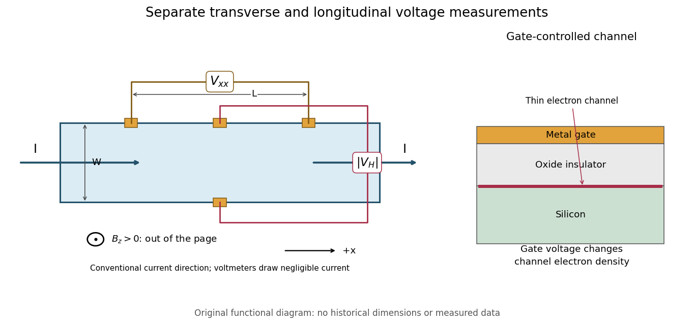
This original functional diagram separates transverse and longitudinal readouts; it does not reproduce the historical device's dimensions. The gate inset explains how a field-effect transistor provides an adjustable two-dimensional electron gas. A longitudinal voltage close to zero is a useful check because accidental longitudinal separation between Hall contacts can otherwise contaminate the transverse measurement.
A Hall bar is a strip with current contacts at its ends and additional voltage contacts along its sides. Opposite-side contacts measure a transverse electric potential difference; same-side contacts at different longitudinal positions measure a longitudinal electric potential difference. Separate voltage leads reduce the influence of current-contact electrical resistance when their input electric currents are negligible.
Voltage contacts separated along the current direction measure longitudinal resistance, even when the device is called a Hall bar. For an approximately uniform rectangular strip, . Transverse contacts measure instead. Shubnikov-de Haas effect oscillations in need not be Hall-resistance plateaus; in the integer quantum Hall effect, longitudinal minima accompany quantized transverse plateaus.
The degeneracy of a Landau level is per resolved internal branch in area . The filling factor varies continuously. Additional localized eigenstates need not carry bulk transport, allowing an integer plateau over an interval of ; a mobility gap need not be an empty spectral gap.[ref]
Quantized Hall Conductance in a Two-Dimensional Periodic Potential by D. J. Thouless and others. p. 405, gaps and localized tails
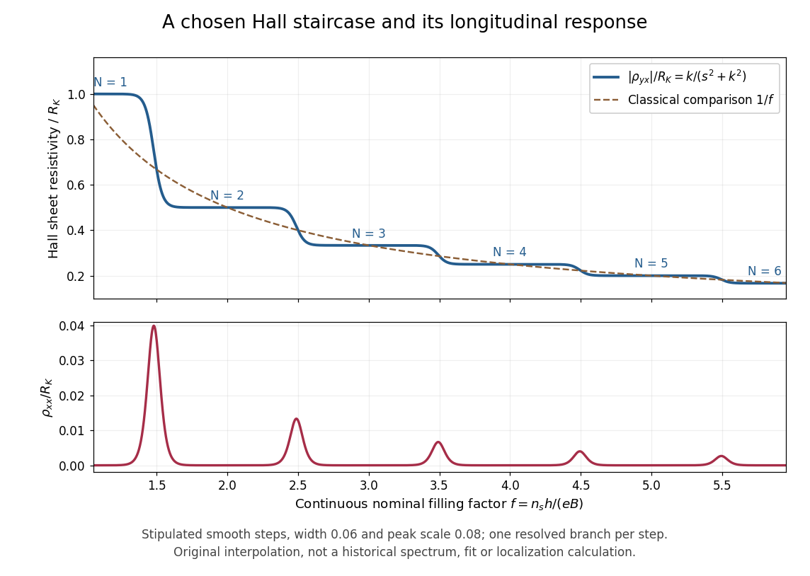
The plot is an original phenomenological construction, not measured data or a calculation of Anderson localization. It stipulates dimensionless transverse sheet conductivity and longitudinal sheet conductivity , with chosen , . Both are measured in units . The quantum Hall conductivity tensor inversion produces and . Regions near , yield plateaus near ; the model alone does not explain their microscopic robustness. Each step represents one resolved branch, without assuming unresolved spin or valley multiplicities.
Choose conventional surface current density along , magnetic field along , and negative electron charge. An isotropic in-plane response has the following sheet conductivity and sheet resistivity tensors for , :These are matrix inverses, rather than componentwise reciprocals. The sheet conductivity has units siemens, the sheet resistivity ohms. With , the sign is , agreeing with the negative Hall coefficient of a single electron species. Contact polarity can reverse the measured voltage sign, so quote the Hall magnitude. For a homogeneous strip of width and longitudinal probe separation , givesAt , , these reduce to and zero. A nonzero transverse sheet resistivity creates no local Joule heating: the antisymmetric contribution cancels in .
For an original nonideal example, choose , and . Then , while the Hall magnitude is below by the relative amount parts per million. An unwanted admixture in the Hall readout would instead introduce approximately . The chosen calculation shows why a small intrinsic tensor correction does not by itself guarantee an accurate contact measurement.
For filled, separated, noninteracting magnetic Bloch bands, the Berry curvature integral over the magnetic Brillouin zone is an integer Chern number , giving . Patches of Berry connection meet through phases with integer windings; continuous gap-preserving changes cannot change . D. J. Thouless, M. Kohmoto, M. P. Nightingale and M. den Nijs developed this band argument; it does not establish the interacting fractional case.[ref]
Quantized Hall Conductance in a Two-Dimensional Periodic Potential by D. J. Thouless and others. pp. 405–407, Kubo formula and phase winding
A quantum Hall edge state is confined across a boundary but can extend along it and carry electric current. B. I. Halperin related these current-carrying boundary states to quantized Hall transport in a disordered two-dimensional system.[ref]
Quantized Hall conductance, current-carrying edge states, and the existence of extended states in a two-dimensional disordered potential by B. I. Halperin. Publisher abstract: transverse confinement, perimeter extension and current
A skipping orbit is the semiclassical path of a charged particle whose cyclotron arcs are repeatedly interrupted by a reflecting boundary. The centre of successive arcs advances along the edge. For electrons in a perpendicular positive , the opposite sides of a strip carry opposite directed motion. A smooth boundary replaces hard reflections by guiding-centre drift; the quantum counterpart is a quantum Hall edge state.
For locally linear electron confinement potential energy , two Zeeman splitting branches cross the same Fermi energy at positions differing by the energy splitting divided by . The expression neglects self-consistent electrostatic screening and exchange interaction enhancement. If the quoted slope is an electrostatic voltage gradient instead of an electron-energy gradient, its magnitude must be multiplied by the elementary charge. A screened compressible quantum Hall edge strip is not a single sharp crossing with an imposed bare slope.
Self-consistent electrostatics allows a partially filled edge Landau level to screen strongly and flatten its effective energy. Such compressible regions alternate with incompressible strips whose chemical potential lies in a gap and across which the potential changes. An externally prescribed unscreened smooth edge misses this redistribution. Temperature, disorder and interactions beyond the electrostatic approximation can change the strip profile.
A depleted potential hill inside a two-dimensional electron gas. In a strong perpendicular magnetic field, closed quantum Hall edge states circulate around it. Coupling these states to propagating edge channels can produce resonant backscattering; Coulomb blockade can substantially alter the single-particle resonance pattern.
A quantum dot is an electron-confining potential well, whereas an antidot is a depleted potential hill. At the same magnetic field, their closed guiding-centre drift has opposite circulation. A series dot needs transmission through two barriers; a side-coupled antidot can connect already propagating quantum Hall edge states and induce backscattering. Both can have discrete energies and charging effects, but a electrical conductance peak or dip depends on lead connectivity rather than solely on the existence of a closed orbit.
A closed antidot edge orbit can tunnel-couple extended channels on opposite edges. When its electrochemical energy aligns with the reservoirs, resonant backscattering reduces conductance from an otherwise transmitting integer plateau. Different connectivity can instead add a transmission path and produce peaks. Gate voltage changes both the orbit and tunnel couplings; charging and spin alter the simplest fixed-area Aharonov-Bohm resonance sequence.
A spin-resolved resonant path adds at most to the electrical conductance of directly transmitted spectator channels. Conversely, resonant transfer into a returning edge removes at most from an otherwise open channel. For an isolated level, reaches one only for equal couplings. Integer offsets follow the channel connectivity and do not follow from a local filling factor alone. temperature, asymmetry, coherent background paths and inelastic processes can change the apparent resonance height and shape.
In an integer-filling charging model, occupied spin-resolved branches can drive approximately charge rearrangements per added flux. Two coupled spin branches can therefore yield near- oscillations. This does not change the elementary single-electron flux quantum and is not guaranteed by counting two independent noninteracting spin spectra alone.
For a fixed effective enclosed area , changing the magnetic flux by changes the single-electron Aharonov-Bohm phase by . Gate-dependent orbit area, spin branches and charging can modify the observed conductance-resonance pattern; the lithographic depleted area need not equal the exact enclosed edge-orbit area.
The fractional quantum Hall effect is quantized transverse sheet conductivity at fractional filling factors, produced by interacting electrons. The Laughlin wavefunction describes the sequence , with odd , including .[ref]
For an original ideal readout example, take a Hall bar on the plateau with negligible longitudinal sheet conductivity. The quantum Hall conductivity tensor inversion givesHere is the von Klitzing constant; denotes transverse electrical resistance, rather than the bulk Hall coefficient. Thus a fractional sheet conductivity corresponds to a larger transverse electrical resistance. The fraction labels a collective quantum state: it does not mean that each electron has acquired one third of its usual electric charge.
An emergent description of correlated electrons in which an even number of statistical flux quanta is attached to each electron. The resulting effective field can turn selected fractional electronic fillings into integer effective fillings. Flux attachment encodes correlations; it is not attachment of literal external magnetic solenoids to individual electrons.
A fully spin-polarized sea of composite fermions has a Fermi wavevector . Near half filling its semiclassical orbit radius depends on the residual effective field, not the full applied field. Matching an orbit diameter to a patterned length can produce transport resonances outside an incompressible fractional Hall state. Multiple pattern periods and random/unpatterned controls test that geometric interpretation. Density inhomogeneity and a soft potential can shift or broaden the response.[ref]
Composite fermions in periodic and random antidot lattices by J. H. Smet and others. pp.3598–3600, Eq.(1) and Figs.1–3
Attach two statistical flux quanta per electron at density . For , and the signed effective filling is . Inversion gives . Integer gives , while gives . Using nonnegative effective filling instead requires explicitly tracking the effective-field sign. At half filling the mean effective field vanishes.
A family of fractional quantum Hall effect fillings obtained by attaching flux quanta and filling effective Landau levels of composite fermions. Positive integers and the relative effective-field direction specify the branch.
Daniel Tsui, Horst Störmer and Arthur Gossard reported the effect in 1982. They grew gallium arsenide–aluminium gallium arsenide layers by molecular beam epitaxy, separating the two-dimensional electron gas from its semiconductor doping. They cut Hall bars and made indium contacts. Low-field measurements established number density and charge carrier mobility. A perpendicular magnetic field sweep measured transverse and longitudinal sheet resistivities at several temperatures. Cooling sharpened the plateau near and the longitudinal minimum at filling factor ; integer plateaus provided an internal comparison. The longitudinal minimum remained finite at the lowest temperature: zero-temperature vanishing was unresolved. This established anomalous transport, without directly measuring excitation electric charge.[ref]
Two-Dimensional Magnetotransport in the Extreme Quantum Limit by Daniel Chee Tsui and others. pp. 1559–1561, sample preparation, Figs. 1–2 and finite longitudinal minimum
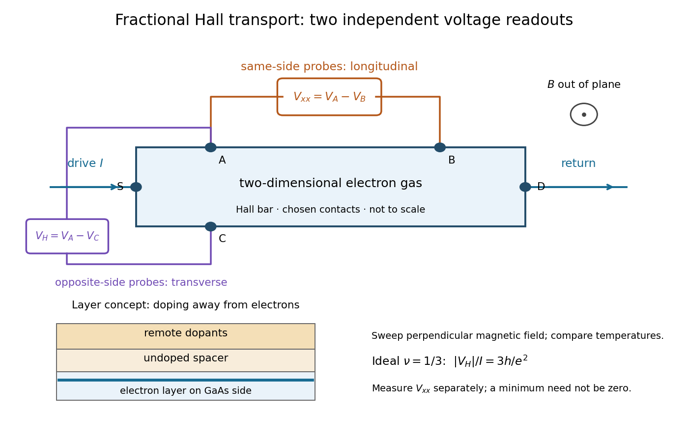
The two readouts test different statements. A single intersection with would also occur on the smooth classical relation at . A quantum Hall plateau instead persists over a magnetic field interval. Comparing transverse and longitudinal signals helps distinguish that plateau from a contact-placement artefact; the quantum Hall conductivity tensor inversion quantifies the contamination when longitudinal sheet resistivity is nonzero.
Later, 1997 shot noise measurements associated with quantum tunnelling at filling factor tested the excitation electric charge separately, finding . That is a different observable from a Hall plateau.[ref]
Observation of the e⁄3 Fractionally Charged Laughlin Quasiparticle by L. Saminadayar and others. Publisher abstract: tunnelling noise and inferred quasiparticle charge
Robert Laughlin's 1983 variational method uses pairwise zeros to suppress close electron encounters within the lowest Landau level. For aligned spin, odd gives fermionic exchange symmetry.[ref]
Here enforces wavefunction normalization, is the magnetic length, and complex coordinates describe electrons in a magnetic field , , with the symmetric gauge. Reversing the orientation conjugates the polynomial without changing probability densities. The Gaussian function confines the wavefunction.
The exchange check is especially simple for two electrons. Writing , exchange sends , so . An aligned two-electron spin state is symmetric, requiring the spatial wavefunction to change sign. Hence works, whereas would give the wrong sign. At a close encounter, the probability density vanishes as : imposes a sixth-order zero, stronger than the quadratic zero at . This is the local geometric mechanism for avoiding a large repulsive Coulomb potential energy.
A useful large- counting outline follows directly from the polynomial. Each complex coordinate has maximum degree . A lowest Landau level orbital proportional to has its areal probability density maximum at , by differentiating its logarithm. This suggests droplet area , neglecting the boundary correction. Dividing by the degeneracy of a Landau level per area, , gives filling factor . This counting is a motivation for the fraction, not an independent proof that the wavefunction minimizes the interacting Hamiltonian.
Consider the original two-electron example obtained by taking in the Laughlin wavefunction, with no additional polynomial for the centre of mass. Introduce , relative complex coordinate , separation , and dimensionless separation . Since , the probability density factorizes:Integrating out leaves an isotropic relative probability density. Define per unit dimensionless area and per unit dimensionless separation:The physical areal probability density is . The probability of a separation between and is . The extra comes from the Jacobian determinant in polar coordinates: a thin annulus has area . Omitting that factor changes the question being answered.
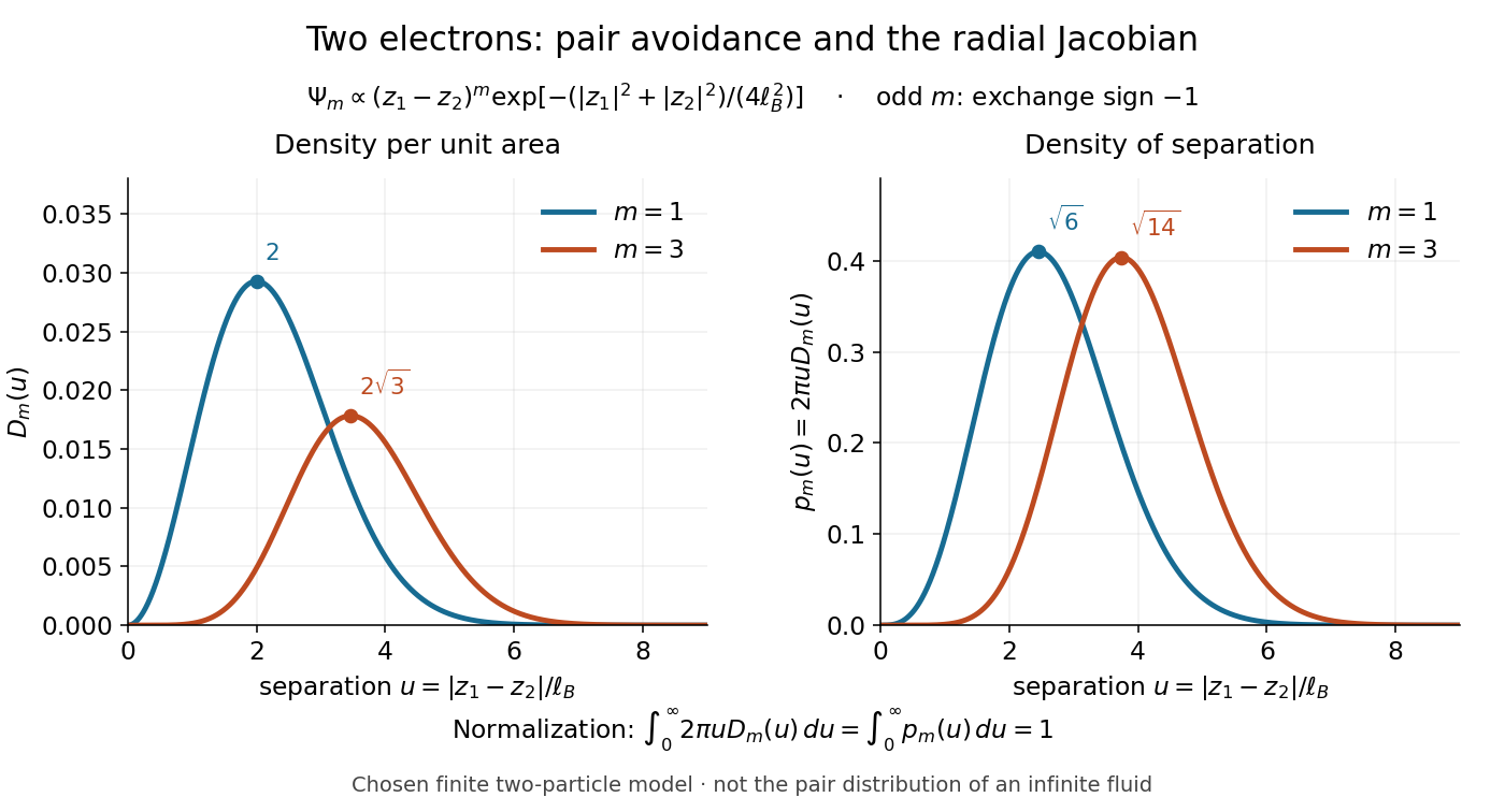
Both wavefunction normalization and the peak shift can be checked exactly. The substitution gives the Gamma function integralFor , logarithmic differentiation givesConsequently the areal maximum lies at , while the most probable separation lies farther out, at . For these are and ; for , and . The same substitution gives , so the root mean square separations are and respectively. The distinction between a probability density maximum and a radial maximum therefore has a directly calculable geometric origin.
This two-electron model explains exchange and pair avoidance. It does not establish a nonzero many-particle spectral gap, an extended quantum Hall plateau, or the topological properties of a fluid in the thermodynamic limit. Those require additional many-electron reasoning and experimental tests.
A quasihole adds one zero at per electron; its local deficit carries positive electric charge .[ref]
Anomalous Quantum Hall Effect: An Incompressible Quantum Fluid with Fractionally Charged Excitations by Robert Laughlin. pp. 1396–1397, Eqs. (13), (15) and screening argument
Here is a transport counting outline, conditional on an incompressible quantum Hall fluid. Inserting one magnetic flux quantum slowly compared with , where is the excitation energy gap, produces a circulating electric field by Faraday's law. The transverse sheet conductivity sends a radial electric current whose time integral has magnitudeThe opposite electric charge moves to the boundary, so the total electric charge remains conserved. The counted deficit belongs to a collective quasiparticle; no individual electron has been cut into pieces. The argument assumes the gapped fluid and its Hall response, and is not a consequence of the finite two-electron normalization integral.
An incompressible quantum Hall fluid has a bulk spectral gap against charged excitations; disorder can localize excess quasiparticles.[ref]
Anomalous Quantum Hall Effect: An Incompressible Quantum Fluid with Fractionally Charged Excitations by Robert Laughlin. pp. 1397–1398, incompressibility and impurity localization
The gyroradius is the radius of the transverse circular motion of a charged particle in a uniform magnetic field. In nonrelativistic classical mechanics, with zero electric field and no other forces, it is , where is the speed perpendicular to the magnetic field. The parallel component of velocity changes the advance of the helix, rather than its transverse radius.
For particles with the same charge-to-mass ratio, rotationally invariant mutual central forces, and a weak uniform magnetic field, a frame with the displayed angular velocity cancels the velocity-dependent magnetic Lorentz force against the Coriolis force. The remaining rotational and magnetic terms are quadratic in . Thus, to first order in the field, the rotating-frame equations coincide with the zero-field equations. This is the classical dynamical basis of Larmor precession; equality is an approximation rather than an exact removal of the magnetic field.
For an axial magnetic field , let . The Lorentz force gives , so is constant. Since magnetic forces do no work and is constant, the transverse speed is constant and . If and , two finite radial turning points confine the motion. If , an outward branch escapes to infinite radius. At equality a marginal escaping branch exists when , but gives a circular orbit instead. The transverse escape velocity threshold is ; motion parallel to the magnetic field cannot provide transverse escape energy.
Under the magnetic-only Lorentz force, planar velocity has constant magnitude and an accumulated phase determined by the time integral of the axial field. For , the planar position involves Fresnel integrals. With initial planar velocity and zero initial position, its limit is . The model prescribes a magnetic-only force; a physical time-dependent field may also produce an induced electric field.
// Target: number-theory.bigb
The magnetic part of the Lorentz force is perpendicular to the particle velocity. Its power is therefore zero, so with no other forces the kinetic energy remains constant. This remains true relativistically because ; a magnetic force can change momentum direction without changing total energy.
A tangential force integral around an instantaneous moving loop is not generally the force work along the actual particle trajectory. For an expanding circular guide, the particle has both radial and tangential velocity; the magnetic radial and tangential powers cancel exactly even when the tangential circulation is nonzero.
For smooth stationary fields on , set and , with all other Christoffel symbols zero. This torsion-free connection makes the equation a geodesic equation with time as affine parameter. Arbitrary smooth fields suffice; a metric realization imposes additional potential conditions.
In uniform perpendicular electric and magnetic fields, the guiding centre of a charged particle drifts with . This velocity is independent of the charge and mass; cyclotron motion is superposed on it.
The covariant force on a charged particle is its charge times the electromagnetic field-strength tensor contracted with its four-velocity. Antisymmetry keeps the four-force orthogonal to that velocity and preserves the rest mass.
A wire carrying current in a magnetic field experiencesThis follows by summing the magnetic part of the Lorentz force over the moving charge carriers.
Consider lab-neutral parallel wires with stationary positive line density and electron line density . Let wire 1's electrons move at along the wire and wire 2's at . The conventional currents are . In the rest frame of wire 2's electrons, wire 1's transformed total linear charge density is . Its radial electric field is .
A wire-2 electron at rest there feels only an electric force. Transforming its transverse force back to the lab divides it by , and multiplying by the lab electron count per length giveswith positive radial direction away from wire 1. The lab-stationary positive charges feel zero net electric force because wire 1 is neutral in their frame. Equal current directions attract; opposite directions repel. Transforming force on each carrier and then counting carriers in the specified frame avoids an incorrect extra length-contraction factor in force per unit length.
In a constant magnetic field with no electric field, a charged relativistic particle moves in a circle in the perpendicular plane. Its angular frequency with respect to proper time iswhereas its angular frequency in an inertial coordinate time is . The orbit radius at speed is
For , choose and parametrize one clockwise orbit by and . Over , the relativistic charged-particle action isThe same formula with applies for either orbit orientation.
In uniform perpendicular electric and magnetic fields, a charged particle's cyclotron orbit has guiding-centre velocityindependent of its charge and mass.
For , the temporal component of the covariant Lorentz-force equation givesThe magnetic field does no work because .
Articles by others on the same topic

The Lorentz force is the force exerted on a charged particle moving through an electromagnetic field. It is named after the Dutch physicist Hendrik Lorentz.



Equation 1.
Lorentz force
. A little suspicious that it bears the name of Lorentz, who is famous for special relativity, isn't it? See: Maxwell's equations require special relativity.